4.1. Entropy

4.1. Entropy#

Overview#

In Module 3, we established the foundations of thermodynamics and explored the concept of enthalpy. We will learn that exothermicity (a negative enthalpy change) often favors spontaneity but does not fully determine it. The missing piece is entropy, a state function that provides crucial insight into the direction of spontaneous change. In this sub-module, we build on those ideas by formally introducing entropy, examining its definition, and understanding its role in the arrow of time for spontaneous processes.

Exothermicity and Spontaneity#

Exothermic reactions are often—but not always—spontaneous. An exothermic process releases heat to its surroundings, corresponding to a negative enthalpy change, \(\Delta H < 0\). While this heat release can drive a process forward, enthalpy alone does not guarantee spontaneity; we must also consider entropy.

An Example: Formation of Liquid Water#

Consider the formation of two moles of liquid water from hydrogen and oxygen gases at 298.15 K and 1 bar:

\[\ce{2H2(g) + O2(g) -> 2H2O(l)}\]

The standard enthalpy change for this reaction is \(-571.66\) kJ for two moles of H\(_2\)O(l), indicating an exothermic process. The reaction releases heat:

Exothermicity in Chemical Terms

In chemical terms, exothermicity is often associated with the formation of stronger chemical bonds in the products than those in the reactants. In this example, forming \(\ce{H-O}\) bonds in water releases more energy than what was required to break \(\ce{H-H}\) and \(\ce{O=O}\) bonds.

It is fortunate that water formation is exothermic, as this makes the reaction more likely to proceed spontaneously under standard conditions.

A Counter Example: Mixing of Two Ideal Gases#

If we mix two ideal gases, such as Ar and Kr, their intermolecular interactions are negligible (ideal-gas behavior), so \(\Delta H = 0\). Nonetheless, mixing occurs spontaneously once the partition is removed.

Show code cell source Hide code cell source

import numpy as np
import matplotlib.pyplot as plt
from scipy.constants import k, eV
from labellines import labelLines
from myst_nb import glue

rng = np.random.default_rng(8251991)

fig, axs = plt.subplot_mosaic([[0, 1]], figsize=(8, 4), constrained_layout=True, sharex=True, sharey=True)

# Before
axs[0].set_title('Before Opening the Stopper')
x_Ar = rng.uniform(-4, 4, 6)
y_Ar = rng.uniform(2, 5, 6)
axs[0].scatter(x_Ar, y_Ar, color='r', label='Ar', s=100)

x_Kr = rng.uniform(-4, 4, 6)
y_Kr = rng.uniform(-5, -2, 6)
axs[0].scatter(x_Kr, y_Kr, color='b', label='Kr', s=100)

# Ar region
axs[0].plot([1, 1], [0, 1], color='k')
axs[0].plot([1, 5], [1, 1], color='k')
axs[0].plot([5, 5], [1, 6], color='k')
axs[0].plot([5, -5], [6, 6], color='k')
axs[0].plot([-5, -5], [6, 1], color='k')
axs[0].plot([-5, -1], [1, 1], color='k')
axs[0].plot([-1, -1], [1, 0], color='k')

# Kr region
axs[0].plot([1, 1], [0, -1], color='k')
axs[0].plot([1, 5], [-1, -1], color='k')
axs[0].plot([5, 5], [-1, -6], color='k')
axs[0].plot([5, -5], [-6, -6], color='k')
axs[0].plot([-5, -5], [-6, -1], color='k')
axs[0].plot([-5, -1], [-1, -1], color='k')
axs[0].plot([-1, -1], [-1, 0], color='k')

# Closed stopper
axs[0].plot([-1.5, 1.5], [0, 0], color='m', lw=2)
axs[0].text(2, 0, "Stopper (closed)", fontsize=10, ha='left', va='center', color='m')
axs[0].set_aspect('equal')
axs[0].axis('off')

# After
axs[1].set_title('After Opening the Stopper')
x_Ar = rng.uniform(-4, 4, 6)
y_Ar_1 = rng.uniform(2, 5, 3)
y_Ar_2 = rng.uniform(-5, -2, 3)
y_Ar = np.concatenate((y_Ar_1, y_Ar_2))
axs[1].scatter(x_Ar, y_Ar, color='r', label='Ar', s=100)

x_Kr = rng.uniform(-4, 4, 6)
y_Kr_1 = rng.uniform(2, 5, 3)
y_Kr_2 = rng.uniform(-5, -2, 3)
y_Kr = np.concatenate((y_Kr_1, y_Kr_2))
axs[1].scatter(x_Kr, y_Kr, color='b', label='Kr', s=100)

axs[1].plot([1, 1], [0, 1], color='k')
axs[1].plot([1, 5], [1, 1], color='k')
axs[1].plot([5, 5], [1, 6], color='k')
axs[1].plot([5, -5], [6, 6], color='k')
axs[1].plot([-5, -5], [6, 1], color='k')
axs[1].plot([-5, -1], [1, 1], color='k')
axs[1].plot([-1, -1], [1, 0], color='k')
axs[1].plot([1, 1], [0, -1], color='k')
axs[1].plot([1, 5], [-1, -1], color='k')
axs[1].plot([5, 5], [-1, -6], color='k')
axs[1].plot([5, -5], [-6, -6], color='k')
axs[1].plot([-5, -5], [-6, -1], color='k')
axs[1].plot([-5, -1], [-1, -1], color='k')
axs[1].plot([-1, -1], [-1, 0], color='k')

# Open stopper
axs[1].plot([-5, -2], [0, 0], color='m', lw=2)
axs[1].text(2, 0, "Stopper (open)", fontsize=10, ha='left', va='center', color='m')
axs[1].axis('off')
axs[1].set_aspect('equal')
axs[1].legend(bbox_to_anchor=(1.05, 1), loc='upper left', borderaxespad=0.)

fig.suptitle(r'$\Delta H = 0$')

glue("gases_before_after", fig, display=False)
plt.close(fig)

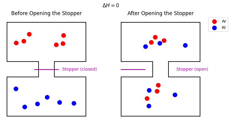
../_images/45e6575af1af233282226f9ab17f21f7233b8d608027785bbaea159f0d4b3508.png — Fig. 26 Mixing of two ideal gases before and after opening the stopper that separates them.#

Even though \(\Delta H = 0\), the process is still spontaneous. If you were shown the “before” and “after” snapshots without additional labels, you would know the natural direction of mixing. This spontaneous behavior underscores that enthalpy alone cannot capture whether a process will occur without additional driving forces. That driving force is related to entropy.

Definition of Entropy#

Entropy#: A state function denoted by \(S\), quantifying the degree of dispersal or spread of energy and matter, thereby predicting the direction of spontaneous change.

First Law for a Reversible Process#

Recall the differential form of the First Law of Thermodynamics for a reversible process in which only \(PV\) work is done on an ideal monatomic gas (\(PV = Nk_{\mathrm{B}}T\) and \(C_V = \tfrac{3}{2}Nk_{\mathrm{B}}\)):

\[\begin{split}\begin{align*} \delta q_{\text{rev}} &= dU - \delta w_{\text{rev}} \\ &= dU + P\,dV \\ &= C_V\,dT + \left[ \left( \frac{\partial U}{\partial V} \right)_T + P \right] dV \\ &= \frac{3}{2} N k_{\mathrm{B}}\,dT + \frac{N k_{\mathrm{B}} T}{V}\,dV. \end{align*}\end{split}\]

Because \(\delta q_{\text{rev}}\) depends on the path, it is an inexact differential.

Dividing by \(T\) to Obtain an Exact Differential#

Observe that if we divide \(\delta q_{\mathrm{rev}}\) by \(T\), the resulting expression becomes exact:

\[\frac{\delta q_{\text{rev}}}{T} \;=\; \frac{3}{2}\,\frac{N k_{\mathrm{B}}}{T} \, dT \;+\; \frac{N k_{\mathrm{B}}}{V}\,dV.\]

Hence, we define entropy \(S\) through the exact differential:

\[dS \;=\; \frac{\delta q_{\text{rev}}}{T}.\]

The change in entropy between two states \(A\) and \(B\) is then:

\[\Delta S \;=\; \int_{A}^{B} \frac{\delta q_{\text{rev}}}{T}.\]

Fundamental Thermodynamic Relation#

From the definition of entropy, we obtain:

\[\delta q_{\text{rev}} \;=\; T\,dS.\]

For a simple closed system with only \(PV\) work,

\[\delta q_{\text{rev}} = dU + P\,dV \;=\; T\,dS \quad\Longrightarrow\quad dU = T\,dS - P\,dV.\]

Here, \(U\) is naturally expressed as a function of the extensive variables \(S\) and \(V\). In systems with additional types of work (e.g., electrical, surface, magnetic), the more general relation becomes:

\[dU \;=\; T\,dS \;+\; \sum_{i} \vec{F}_{i}\cdot d\vec{x}_{i}.\]

Natural Variables

A state function’s natural variables are those that appear as independent variables in its total differential. For internal energy \(U\), the natural variables are \(S\) and \(V\) for a simple system with only \(PV\) work.