2.5. Particle in a Box#
Overview#
This section discusses the quantum mechanical treatment of a particle in a box, along with the derivation of key thermodynamic properties using the partition function. We begin with a review of the one-dimensional case, generalize to three dimensions, and then show how the classical partition function emerges in the high-temperature or large-volume limit.
Review of the Particle in a Box#
Particle in a One-Dimensional Box#
Show code cell source
import numpy as np
import matplotlib.pyplot as plt
from mpl_toolkits.mplot3d.art3d import Poly3DCollection
from scipy.constants import k, eV
from labellines import labelLines
from myst_nb import glue

fig, axs = plt.subplot_mosaic([[0]], figsize=(4, 4))

# Plot a one-dimensional box
axs[0].plot([-0.5, -0.5], [18, 0], color='black', zorder=2.5, lw=4)
axs[0].plot([-0.5, 0.5], [0, 0], color='black', zorder=2.5, lw=4)
axs[0].plot([0.5, 0.5], [0, 18], color='black', zorder=2.5, lw=4)

# Plot the energy levels (blue lines)
for n in range(1, 5):
    energy = axs[0].plot([-0.5, 0.5], [n**2, n**2], color='blue', label=r'$E_{%d}$' % n)
    labelLines(energy, xvals=[-1/6], zorder=2.5)

# Plot the wavefunctions (red curves)
x = np.linspace(-0.5, 0.5, 100)
for n in range(1, 5):
    wavefunction = axs[0].plot(x, np.sin(n * np.pi * (x + 0.5)) + n**2, color='red', label=r'$\psi_{%d}$' % n)
    labelLines(wavefunction, xvals=[1/6], zorder=2.5)

axs[0].set_xlabel('Position')
axs[0].set_ylabel('Energy')
axs[0].set_xticks([-0.5, 0, 0.5])
axs[0].set_xticklabels([r'$-L/2$', r'$0$', r'$L/2$'])
axs[0].set_yticks([])
axs[0].spines['top'].set_visible(False)
axs[0].spines['right'].set_visible(False)
axs[0].spines['left'].set_visible(False)

plt.tight_layout()
glue("particle_in_a_box", fig, display=False)
plt.close(fig)
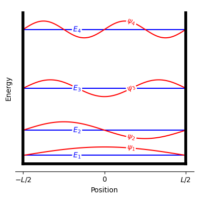
Fig. 16 Boundary conditions, energy levels, and wavefunctions for a particle in a one-dimensional box. The energy levels \(E_n\) are shown as horizontal blue lines, while the wavefunctions \(\psi_n\) are shown as red curves.#
For a particle in a one-dimensional box of length \(L\), the quantized energy levels are
where \(h\) is Planck’s constant, \(m\) is the particle mass, and \(n\) is a positive integer.
Particle in a Three-Dimensional Box#
In three dimensions, the energy levels become
where \(n_x\), \(n_y\), and \(n_z\) are positive integers, and \(L_x\), \(L_y\), and \(L_z\) are the respective side lengths of a rectangular box.
Particle in a Cube#
When the box is a cube of side \(L\), \(L_x = L_y = L_z = L\). The energy then simplifies to
where \(V = L^3\) is the volume of the cube.
Partition Function for a Particle in a Cube#
The partition function for a single particle in a three-dimensional cube is:
Defining \(\alpha = \beta h^2 / (8 m V^{2/3})\), we can rewrite \(q\) as:
Approximation of the Sum#
For large \(T\) or large \(L\), the sum \(\sum_{n=1}^{\infty} e^{-\alpha n^2}\) can be approximated by an integral:
Substituting \(\alpha = \beta h^2/(8 m V^{2/3})\) gives:
We often define the thermal de Broglie wavelength \(\Lambda\) as
What is the thermal de Broglie wavelength?
The thermal de Broglie wavelength, \(\Lambda\), is a characteristic length scale that quantifies the quantum mechanical “spread” of a particle’s wavefunction at a given temperature. When the average distance between particles is much greater than \(\Lambda\), the system behaves classically, allowing particles to be treated as distinguishable. Conversely, if the interparticle spacing is on the order of \(\Lambda\) or smaller, quantum effects become significant, and the particles must be treated as indistinguishable.
Hence,
So the single-particle partition function becomes
Partition Function for \(N\) Particles in a Cube#
For \(N\) identical, non-interacting, indistinguishable particles, the total partition function \(Q\) is
The factor of \(N!\) corrects for the indistinguishability of the particles (i.e., permutations of identical particles do not lead to new states).
Ensemble Averages for \(N\) Particles in a Cube#
Natural Logarithm of the Partition Function#
Taking the logarithm of \(Q\):
Often, the Stirling approximation (\(\ln N! \approx N \ln N - N\)) is used for large \(N\).
Internal Energy#
The internal energy \(U\) is found via:
Important
This result matches the equipartition theorem, implying each of the three translational degrees of freedom contributes \(\frac{1}{2} k_{\text{B}} T\) per particle. Note that \(U\) is independent of the volume \(V\) because the particles do not interact.
Heat Capacity at Constant Volume#
From \(U = \frac{3}{2} N k_{\text{B}} T\), it follows that:
Important
This temperature-independent \(C_V\) is a hallmark of an ideal (monatomic) gas.
Pressure#
To find the pressure, we use:
recovering the ideal gas law.
Translational Partition Function#
Because the energy levels of a particle in a box primarily account for translational motion, the partition function
is called the translational partition function. It underpins much of our classical description of gases when \(\Lambda \ll\) (typical particle spacing), ensuring that quantum effects are negligible at normal densities and temperatures.