3.2. Applications of the First Law#
Overview#
This section explores how to apply the First Law of Thermodynamics to various thermodynamic processes. We begin by clarifying key process definitions, then outline a step-by-step method for using the First Law under different constraints, and end with a microscopic interpretation that connects probability distributions of microstates with heat exchange.
Thermodynamic Processes#
- Quasi-static process#
A process carried out infinitesimally slowly so that the system remains nearly in equilibrium at all times. Each intermediate state is well-defined thermodynamically.
- Reversible process#
An idealized process that is (1) quasi-static and (2) free of dissipative effects, meaning it can be reversed with no net change to the system or surroundings.
- Irreversible process#
Any process that violates one or more of the conditions for reversibility (e.g., too rapid, frictional, or dissipative).
How to Apply the First Law of Thermodynamics#
The First Law states:
where \(dU\) is the change in internal energy, \(\delta q\) is the heat added to the system, and \(\delta w\) is the work done by the system. To make this law more useful for specific processes, follow the steps below.
Step 1. Choose Two Independent Variables
Convenience: Which variables are easiest to control with your experimental setup?
Necessity: Which variables can you reliably measure or keep constant?
Curiosity: Which variables are most relevant to the phenomenon you wish to explore?
Typically, two independent variables are sufficient (e.g., \(P\) and \(T\), or \(V\) and \(T\)).
Step 2. Rewrite the First Law
Express \(\delta q\) and \(\delta w\) in terms of infinitesimal changes in your chosen variables (\(X_1\) and \(X_2\)):
\[\delta q \;=\; \left(\frac{\partial U}{\partial X_1}\right)_{X_2} dX_1 \;+\; \left(\frac{\partial U}{\partial X_2}\right)_{X_1} dX_2 \;+\;\dots\]Include work appropriately. For \(P\)-\(V\) work, \(\delta w = -P\, dV\).
Step 3. Apply Constraints
Constant Variables:
Isobaric (\(dP=0\)), Isochoric (\(dV=0\)), Isothermal (\(dT=0\)).
Adiabatic:
If the boundary is thermally insulating, \(\delta q = 0\).
“Adiabatic” means no heat transfer, but the system may still perform work.
Step 4. Define the System
Specify an equation of state if known (e.g., \(PV=nRT\) for an ideal gas).
Use the equation of state to evaluate partial derivatives—e.g., \(\left(\frac{\partial U}{\partial V}\right)_T\)—that appear in your expression for \(\delta q\).
Step 5. Integrate the First Law
Integrate the differential relationships to link total heat (\(q\)) or work (\(w\)) to finite changes in state variables.
Even real (irreversible) processes can be analyzed by approximating or comparing to ideal, reversible paths.
Why It Matters
Different process constraints (isobaric, isochoric, isothermal, adiabatic) dictate how heat, work, and changes in state variables interrelate. Mastering these constraints reveals how energy flows and how measurable quantities (e.g., temperature, volume, pressure) change under specific conditions.
Example: Using \(V\) and \(T\) as Independent Variables#
For many systems—especially gases—choosing \(V\) and \(T\) can simplify calculations.
First Law in Terms of \(V\) and \(T\)#
Starting from
rewrite \(dU\) with a total differential:
Thus,
If the system is an ideal gas, \(\left(\frac{\partial U}{\partial V}\right)_T = 0\) because \(U\) depends only on \(T\). For a monoatomic ideal gas,
Process Constraints#
Constraint |
Condition |
Resulting \(\delta q\) |
|---|---|---|
Isochoric |
\(dV = 0\) |
\(\delta q = C_V\, dT\) |
Isothermal |
\(dT = 0\) |
\(\delta q = P\, dV\) |
Adiabatic |
\(\delta q = 0\) |
\(C_V\, dT = -P\, dV\) |
Integrations Under Specific Constraints#
Isochoric (\(dV = 0\))
\[\delta q = C_V\, dT \quad \Longrightarrow \quad q = \int_{T_1}^{T_2} C_V \, dT = \frac{3}{2} N k_B \,\Delta T.\]Isothermal (\(dT = 0\)) Since \(\delta q = P\, dV\),
\[q = \int_{V_1}^{V_2} \frac{N k_B T}{V} \, dV = N k_B T \ln\!\bigl(\tfrac{V_2}{V_1}\bigr).\]Adiabatic (\(\delta q = 0\))
\[C_V\, dT = -P\, dV \quad \Longrightarrow \quad \int_{T_1}^{T_2} C_V\, \frac{dT}{T} = - \int_{V_1}^{V_2} \frac{N k_B}{V}\, dV.\]After integration,
\[T_1 V_1^{2/3} = T_2 V_2^{2/3}.\]
Microscopic Interpretation of the First Law#
From a statistical mechanics perspective, the internal energy is
where \(p_i\) is the probability of occupying the \(i\)-th microstate with energy \(E_i\). The total differential can be written as
For a closed system (constant \(N\)), and noting that
we identify pressure as
Hence,
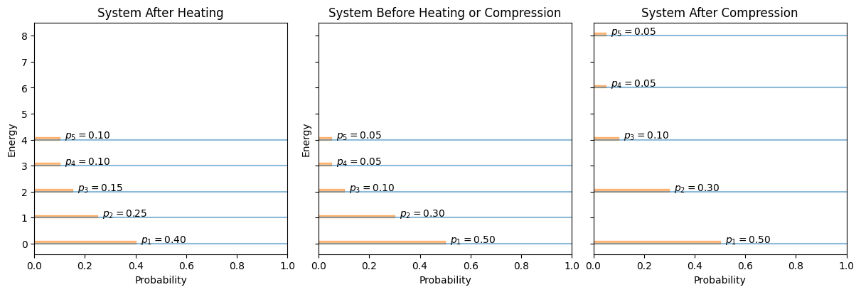
Comparing with \(\delta q = \sum_{i=1}^M E_i\, dp_i\), we see that heat is the energy exchange via changing probabilities \(p_i\), while work is the energy exchange via changes in the microstate energies themselves (e.g., volume compression).
Show code cell source
import numpy as np
import matplotlib.pyplot as plt
from scipy.constants import k, eV
from labellines import labelLines
from myst_nb import glue

# This code illustrates how microstate energies and probabilities change under heating or compression.

N_microstates = 5
E_microstates = np.array([0, 1, 2, 3, 4])
P_microstates = np.array([0.5, 0.3, 0.1, 0.05, 0.05])
P_microstates /= P_microstates.sum()

fig, axs = plt.subplots(1, 3, figsize=(12, 4), constrained_layout=True, sharex=True, sharey=True)
# ax.set_title('Schematic of Microstates')

axs[1].set_title('System Before Heating or Compression')

for i in range(N_microstates):
    axs[1].plot([0, 1], [E_microstates[i], E_microstates[i]], color='C0', alpha=0.5)
    axs[1].fill_betweenx([E_microstates[i], E_microstates[i] + 0.1], 0, P_microstates[i], color='C1', alpha=0.5)
    axs[1].text(P_microstates[i] + 0.02, E_microstates[i] + 0.05, f'$p_{i+1}={P_microstates[i]:.2f}$', fontsize=10, ha='left')
axs[1].set_xlabel('Probability')
axs[1].set_ylabel('Energy')
axs[1].set_xlim(0, 1)

axs[0].set_title('System After Heating')

P_microstates_heated = np.array([0.4, 0.25, 0.15, 0.1, 0.1])  # Example probabilities after heating

# Normalize the probabilities (just in case)
P_microstates_heated /= np.sum(P_microstates_heated)

for i in range(N_microstates):
    axs[0].plot([0, 1], [E_microstates[i], E_microstates[i]], color='C0', alpha=0.5)
    axs[0].fill_betweenx([E_microstates[i], E_microstates[i] + 0.1], 0, P_microstates_heated[i], color='C1', alpha=0.5)
    axs[0].text(P_microstates_heated[i] + 0.02, E_microstates[i] + 0.05, f'$p_{i+1}={P_microstates_heated[i]:.2f}$', fontsize=10, ha='left')

axs[2].set_title('System After Compression')

E_microstates_compressed = np.array([0, 2, 4, 6, 8])  # Example energies after compression

for i in range(N_microstates):
    axs[2].plot([0, 1], [E_microstates_compressed[i], E_microstates_compressed[i]], color='C0', alpha=0.5)
    axs[2].fill_betweenx([E_microstates_compressed[i], E_microstates_compressed[i] + 0.1], 0, P_microstates[i], color='C1', alpha=0.5)
    axs[2].text(P_microstates[i] + 0.02, E_microstates_compressed[i] + 0.05, f'$p_{i+1}={P_microstates[i]:.2f}$', fontsize=10, ha='left')

# Add labels to the axes
axs[0].set_xlabel('Probability')
axs[1].set_xlabel('Probability')
axs[2].set_xlabel('Probability')
axs[0].set_ylabel('Energy')
axs[0].set_xlim(0, 1)
axs[1].set_xlim(0, 1)
axs[2].set_xlim(0, 1)

glue("microstates_energy_probabilities", fig, display=False)
plt.close(fig)

Fig. 24 Schematic of microstate energies (vertical) and probabilities (horizontal). Heating changes the distribution \(\{p_i\}\); compression shifts microstate energies \(E_i\).#
By connecting heat transfer to probability shifts and work to energy-level changes, the microscopic picture of the First Law becomes clearer: energy enters or leaves the system either by rearranging how likely each microstate is (heat) or by shifting the energy of each microstate itself (work).
