3.3. Enthalpy#
Overview#
Enthalpy \(H\) is a thermodynamic potential particularly convenient for processes at constant pressure, which is common in chemistry.
Defining Enthalpy#
Consider the first-law expression when \(T\) and \(P\) are the independent variables:
At constant pressure, this becomes:
Define the heat capacity at constant pressure, \(C_P\):
We seek a state function \(H\) such that
This motivates the definition of enthalpy:
Demonstrating That \(H\) Yields \(\delta q_P\)
By substituting \(H = U + PV\), Equation (24), into \(\delta q_P = \left(\partial H / \partial T\right)_P dT\), Equation (23):
This matches Equation (22), thus confirming that \(\delta q_P = \mathrm{d}H\) at constant pressure.
Measuring Enthalpy and Enthalpy Changes#
At constant pressure, the heat absorbed or released by a process is equal to the change in enthalpy of the system:
If \(C_P\) is approximately constant over the temperature range \(\Delta T = T_f - T_i\), then
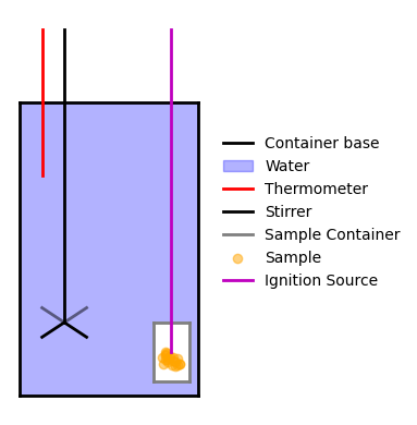
A typical way to measure \(\Delta H\) experimentally is via calorimetry. Below is a schematic of a simple calorimeter:
Show code cell source
import numpy as np
import matplotlib.pyplot as plt
from scipy.constants import k, eV
from labellines import labelLines
from myst_nb import glue

fig = plt.figure(figsize=(4, 4))

# Container
plt.plot([0, 2], [0, 0], 'k-', lw=2, label='Container base')
plt.plot([0, 2], [2, 2], 'k-', lw=2)
plt.plot([0, 0], [0, 2], 'k-', lw=2)
plt.plot([2, 2], [0, 2], 'k-', lw=2)

# Water
plt.fill_between([0, 2], 0, 2, color='blue', alpha=0.3, label='Water')

# Thermometer
plt.plot([0.25, 0.25], [1.5, 2.5], 'r-', lw=2, label='Thermometer')

# Stirrer
plt.plot([0.5, 0.5], [0.5, 2.5], 'k-', lw=2, label='Stirrer')
plt.plot([0.25, 0.5, 0.75], [0.4, 0.5, 0.4], 'k-', lw=2)
plt.plot([0.25, 0.5, 0.75], [0.6, 0.5, 0.6], 'k-', lw=2, alpha=0.5)

# Sample container
plt.plot([1.5, 1.9], [0.1, 0.1], 'C7-', lw=2, label='Sample Container')
plt.plot([1.5, 1.9], [0.5, 0.5], 'C7-', lw=2)
plt.plot([1.5, 1.5], [0.1, 0.5], 'C7-', lw=2)
plt.plot([1.9, 1.9], [0.1, 0.5], 'C7-', lw=2)

plt.fill_between([1.5, 1.9], 0.1, 0.5, color='white')

# Sample inside container
np.random.seed(42)  # For reproducibility
x_sample = np.random.uniform(1.6, 1.8, 20)
y_sample = np.random.uniform(0.2, 0.3, 20)
plt.scatter(x_sample, y_sample, color='orange', alpha=0.5, label='Sample')

# Ignition source
plt.plot([1.7, 1.7], [0.3, 2.5], 'm-', lw=2, label='Ignition Source')

plt.legend(bbox_to_anchor=(1.05, 0.5), loc='center left', borderaxespad=0., frameon=False)
plt.axis('off')
plt.tight_layout()
glue("calorimeter_diagram", fig, display=False)
plt.close(fig)

Fig. 25 A simplified calorimeter. The process occurs in the sample container, which transfers heat to or from the surrounding water at constant pressure. The thermometer and stirrer ensure accurate, uniform temperature readings.#
Build Your Own Calorimeter
Question: How might you build a rudimentary calorimeter with a Styrofoam cup?
Think about a simple chemical reaction in your kitchen.
Hint
Consider a reaction that involves dissolving a solid in water. You could use a thermometer to measure the temperature change.
Defining Common Enthalpy Changes#
Standard Conditions#
Standard conditions are defined as \(P^\circ = 1\text{ bar}\). Reference databases—e.g., the NIST-JANAF Thermochemical Tables and Active Thermochemical Tables—often document properties at \(T = 25^\circ C\) (298.15 K).
Standard Enthalpy of Formation#
The standard enthalpy of formation, \(\Delta H_f^\circ\), is the enthalpy change when 1 mole of a compound is formed from its constituent elements in their standard states.
The standard state of an element is its most stable form at \(P^\circ = 1\text{ bar}\) (and a specified \(T\)).
By convention, \(\Delta H_f^\circ\) for an element in its standard state is zero.
Standard State |
Elements |
|---|---|
Monatomic ideal gas |
He, Ne, Ar, Kr, Xe, Rn |
Homonuclear diatomic ideal gas |
H, N, O, F, Cl |
Liquid |
Br, Hg |
Solid |
All other elements |
Crystal Structure |
Elements |
|---|---|
Body-centered cubic |
Alkali metals (Li, Na, K, Rb, Cs), Ba, group 5 transition metals (V, Nb, Ta), group 6 transition metals (Cr, Mo, W), Mn, Fe, & Eu |
Hexagonal |
Be, Mg, group 3 transition metals (Sc, Y, Lu), group 4 transition metals (Ti, Zr, Hf), Tc, Re, Ru, Os, Co, group 12 transition metals (Zn, Cd), Tl, C (graphite), Se, Te, most lanthanides (La, Ce, Pr, Nd, Pm, Gd, Tb, Dy, Ho, Er, Tm) |
Face-centered cubic |
Ca, Sr, Rh, Ir, group 10 transition metals (Ni, Pd, Pt), group 11 transition metals (Cu, Ag, Au), Al, Si (diamond cubic), Ge (diamond cubic), Pb, Yb |
Rhombohedral |
B, As, Sb, Bi, Sm |
Orthorhombic |
Ga, P (black), S, I, U, and others |
Body-centered tetragonal |
In, Sn (\(\beta\), white) |
Simple cubic |
Po |
Standard Enthalpy of Reaction#
The standard enthalpy of reaction, \(\Delta H_{\mathrm{rxn}}^\circ\), is the enthalpy change when a reaction is carried out under standard conditions. Mathematically:
where \(\nu_p\) and \(\nu_r\) are stoichiometric coefficients of products and reactants, respectively.
Hess’s Law & Standard Enthalpies of Formation
Hess’s Law: Enthalpy changes are additive and path independent. Consequently,
For example, consider the steam–methane reforming reaction:
Directly:
Alternatively, break each species into formation (or reverse formation) reactions from the elemental forms, then sum their enthalpy changes:
Breakdown of the Steam–Methane Reforming Reaction
Either approach gives the same result, thanks to Hess’s Law.
