2.7. Linear Rigid Rotor

Overview

This section covers the quantum mechanical treatment of a linear rigid rotor (e.g., a diatomic molecule) and shows how to derive thermodynamic properties from its rotational partition function.

Review of the Linear Rigid Rotor

Show code cell source Hide code cell source

import numpy as np
import matplotlib.pyplot as plt
from mpl_toolkits.mplot3d.art3d import Poly3DCollection
from scipy.constants import k, eV
from labellines import labelLines
from myst_nb import glue

fig, axs = plt.subplot_mosaic([[0]], figsize=(4, 4))

# Plot the energy levels (blue lines)
for J in range(0, 3):
    g_J = 2 * J + 1
    x_min = -0.04 - 0.1 * (g_J - 1) / 2
    for i in range(g_J):
        # Plot each degenerate sub-level horizontally
        if i == (g_J - 1) / 2:
            energy_line = axs[0].plot(
                [x_min, x_min + 0.08], 
                [J * (J + 1), J * (J + 1)], 
                color='blue',
                label=r'$E_{%d}$' % J
            )
        else:
            axs[0].plot(
                [x_min, x_min + 0.08], 
                [J * (J + 1), J * (J + 1)], 
                color='blue'
            )
        x_min += 0.1
    # Label only one line at each J for clarity
    labelLines(energy_line, zorder=2.5)

axs[0].set_ylabel('Energy (arb. units)')
axs[0].set_xticks([])
axs[0].set_yticks([])
axs[0].spines['top'].set_visible(False)
axs[0].spines['bottom'].set_visible(False)
axs[0].spines['right'].set_visible(False)
axs[0].spines['left'].set_visible(False)

plt.tight_layout()
glue('linear_rigid_rotor_energy_levels', fig, display=False)
plt.close(fig)

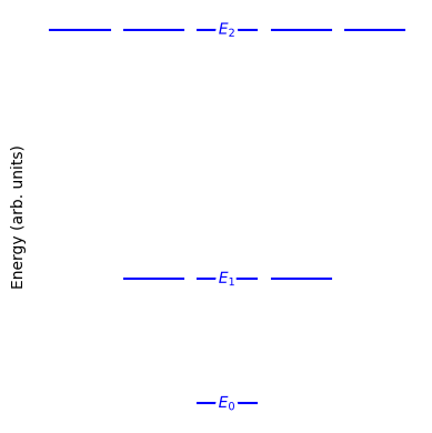
Fig. 21 Energy levels for a linear rigid rotor. The level labeled \(E_J\) has degeneracy \(g_J = 2J + 1\). For example, the \(J=2\) level is split into five degenerate microstates corresponding to \(m = -2, -1, 0, 1, 2\).

For a rigid, linear rotor of moment of inertia \(I\), the energy levels are:

\[E_J \;=\; \frac{\hbar^2}{2I}\,J\bigl(J+1\bigr) \quad\text{for}\quad J = 0, 1, 2, \dots\]

Here, \(\hbar\) is the reduced Planck constant, and \(g_J = 2J + 1\) is the degeneracy of level \(E_J\).

Physical Significance of the Moment of Inertia

The moment of inertia \(I\) measures how mass is distributed around the rotation axis. For a diatomic molecule of atoms A and B,

\[ I \;=\; \mu\,r^2, \quad \mu = \frac{m_A\,m_B}{m_A + m_B},\]

where \(r\) is the bond length and \(\mu\) is the reduced mass of the two atoms.

Partition Function for a Linear Rigid Rotor

In the canonical ensemble, the rotational partition function is:

\[q_{\mathrm{rot}} \;=\; \sum_{i=0}^\infty e^{-\beta E_i} \;=\; \sum_{J=0}^\infty g_J \, e^{-\beta\,E_J} \;=\; \sum_{J=0}^\infty (2J+1)\,\exp\!\Bigl[-\beta \,\frac{\hbar^2}{2I}\,J(J+1)\Bigr].\]

Summation vs. Levels

• Sum over \(i\): sums over individual microstates (each degenerate sub-level).

• Sum over \(J\): reorganizes the sum by energy level \(E_J\), factoring in the degeneracy \(g_J = 2J+1\).

High-Temperature Approximation

When \(k_\mathrm{B} T \gg \frac{\hbar^2}{2I}\), we can approximate the discrete sum by converting it into an integral. Let us set

\[x \;=\; J(J+1), \quad dx \;=\; (2J+1)\,dJ.\]

Hence,

\[q_{\mathrm{rot}} \;\approx\; \int_{0}^{\infty} (2J+1)\,\exp\Bigl[-\beta \,\frac{\hbar^2}{2I}\,J(J+1)\Bigr]\;dJ \;=\; \int_{x=0}^{\infty} \exp\Bigl[-\beta \,\tfrac{\hbar^2}{2I}\,x\Bigr]\;dx.\]

Evaluating this integral,

\[\int_{0}^{\infty} \exp\Bigl[-\beta \,\tfrac{\hbar^2}{2I}\,x\Bigr]\;dx \;=\; \frac{1}{\beta \,\frac{\hbar^2}{2I}} \;=\; \frac{2I\,k_\mathrm{B} T}{\hbar^2}.\]

We define the rotational temperature \(\Theta_{\mathrm{rot}}\) by

\[\Theta_{\mathrm{rot}} \;=\; \frac{\hbar^2}{2k_{\mathrm{B}}\,I}.\]

Thus, for a heteronuclear diatomic rotor (symmetry factor \(\sigma = 1\)),

\[q_{\mathrm{rot}} \;\approx\; \frac{2I\,k_\mathrm{B} T}{\hbar^2} \;=\; \frac{T}{\Theta_{\mathrm{rot}}}.\]

Symmetry Factor \(\sigma\)

For homonuclear diatomics, or other symmetric linear rotors, identical orientations in space might be indistinguishable, leading to \(\sigma=2\). This modifies the partition function to

\[q_{\mathrm{rot}} \;\approx\; \frac{T}{\sigma\,\Theta_{\mathrm{rot}}}.\]

Whether or not you include \(\sigma\) depends on the level of detail needed (e.g., for absolute entropy calculations).

Ensemble Averages

Natural Logarithm of the Partition Function

From the high-\(T\) approximation (with \(\sigma=1\) for simplicity),

\[\ln q_{\mathrm{rot}} \;=\; \ln \Bigl(\tfrac{T}{\Theta_{\mathrm{rot}}}\Bigr) \;=\; \ln T \;-\;\ln \Theta_{\mathrm{rot}}.\]

Internal Energy

The (rotational) internal energy \(U_{\mathrm{rot}}\) is given by

\[U_{\mathrm{rot}} \;=\; - \left(\frac{\partial \ln q_{\mathrm{rot}}}{\partial \beta}\right)_{N,V} \;=\; k_{\mathrm{B}}\,T^2 \left(\frac{\partial \ln q_{\mathrm{rot}}}{\partial T}\right)_{N,V}.\]

Since \(\ln q_{\mathrm{rot}} = \ln T - \ln \Theta_{\mathrm{rot}},\) we get

\[\frac{\partial \ln q_{\mathrm{rot}}}{\partial T} \;=\; \frac{\partial}{\partial T}\bigl(\ln T\bigr) \;=\; \frac{1}{T}.\]

Hence,

\[U_{\mathrm{rot}} \;=\; k_{\mathrm{B}} \, T.\]

Heat Capacity at Constant Volume

The rotational contribution to the heat capacity is

\[C_V^{(\mathrm{rot})} \;=\; \left(\frac{\partial U_{\mathrm{rot}}}{\partial T}\right)_{N,V} \;=\; k_{\mathrm{B}}.\]

Physically, this means one linear rotor contributes \(k_{\mathrm{B}}\) to the heat capacity in the classical (high-\(T\)) limit, corresponding to its two rotational degrees of freedom (each contributes \(\tfrac{1}{2}k_{\mathrm{B}}\)).

Note

In a more rigorous quantum treatment (and for lower temperatures), the partition function and the resulting averages must use the full sum over \(J\). At sufficiently low \(T\), only the \(J=0\) and \(J=1\) levels are significantly populated, which reduces the effective heat capacity below \(k_\mathrm{B}\).