2.1. Introduction to Statistical Mechanics

Overview

        ---
config:
  layout: elk
  look: handDrawn
  theme: neutral

---
flowchart LR
  %% Beginnings and ending
  CM([Classical mechanics])
  QM([Quantum mechanics])
  Th([Thermodynamics])

  %% Processes
  KT[[Kinetic theory]]
  SM[[Statistical mechanics]]

  %% Inputs/Outputs
  StateCM[/"<i>r<sup>N</sup></i>, <i>p<sup>N</sup></i>"/]
  StateQM[/"&Psi;(<i>r<sup>N</sup></i>)"/]
  
  %% Decision
  LimitCM{"Classical limit?"}

  subgraph Microscopic World
    QM
    CM
    StateCM
    StateQM
    LimitCM
  end
  
  subgraph Bridges
    KT
    SM
  end
  
  subgraph Macroscopic World
    Th
  end
  
  CM --> StateCM
  StateCM --> KT --> Th
  StateCM --> SM --> Th
  
  QM --> LimitCM
  LimitCM -- Yes --> CM
  LimitCM -- No --> StateQM --> SM
    

Macroscopic Properties as Expected Values of Microscopic Properties

A core principle of statistical mechanics is that macroscopic thermodynamic properties can be interpreted as statistical averages (or expected values) of microscopic properties.

Arithmetic Average vs. Expected Value

In basic statistics, an arithmetic average \(\bar{X}\) of a set of numbers \(X = \{ X_1, X_2, \ldots, X_M \}\) is:

\[\bar{X} = \frac{1}{M} \sum_{i=1}^M X_i.\]

Example of an Arithmetic Average

The arithmetic average of \(X = \{ 1, 2, 2, 3, 3, 3, 4, 4, 4, 4 \}\) is

\[\bar{X} = \frac{1}{10} \left(1 + 2 + 2 + 3 + 3 + 3 + 4 + 4 + 4 + 4\right) = 3.\]

In statistical mechanics, we often deal with an expected value, which accounts for the probabilities \(p_i\) of different microscopic states or outcomes. The expected value of a random variable \(X\) is:

(11)\[\langle X \rangle = \sum_{i=1}^M X_i \, p_i,\]

where \(p_i\) is the probability of the \(i\)-th value \(X_i\), and the sum runs over all possible microstates.

Example of an Expected Value

If \(X\) takes the values \(\{1, 2, 3, 4\}\) with probabilities \(p = \{0.1, 0.2, 0.3, 0.4\}\), then

\[\langle X \rangle = 1 \times 0.1 + 2 \times 0.2 + 3 \times 0.3 + 4 \times 0.4 = 3.\]

Expected Value of the Number of Tails in 100 Fair Coin Flips

Let \(X_\text{heads} = 0\) and \(X_\text{tails} = 1\). For one flip,

\[\langle X \rangle_1 = 0 \times 0.5 + 1 \times 0.5 = 0.5.\]

Hence, in 100 flips,

\[\langle X \rangle_{100} = 100 \times 0.5 = 50.\]

Expected Value of the Number of Sixes in 300 Fair Die Rolls

Let \(X_\text{six} = 1\) and \(X_\text{not-six} = 0\). Then, for one roll,

\[\langle X \rangle_1 = 1 \times \frac{1}{6} + 0 \times \frac{5}{6} = \frac{1}{6}.\]

For 300 rolls,

\[\langle X \rangle_{300} = 300 \times \frac{1}{6} = 50.\]

Table 6 Statistical Variables and Their Definitions

Statistical Variable	Statistical Mechanical Definition
\(M\)	Number of microscopic states (microstates)
\(i\)	Index of a microstate
\(X_i\)	Value of a microscopic property in the \(i\)-th microstate
\(\langle X \rangle\)	Expected (ensemble) average of \(X\)
\(p_i\)	Probability of finding the system in the \(i\)-th microstate

In thermodynamics, typical \(X\) values might be the internal energy, enthalpy, or other measurable properties. We will see how to compute such properties by defining appropriate probabilities \(p_i\) for the relevant ensemble.

Ensembles of Microstates

Ensemble

The set of all possible microstates of a system consistent with the macroscopic properties of the system.

Microcanonical ensemble

All microstates have the same number of particles, volume, and energy \(\left( N, V, E \right)\).

Canonical ensemble

All microstates have the same number of particles, volume, and temperature \(\left( N, V, T \right)\).

Grand canonical ensemble

All microstates have the same chemical potential, volume, and temperature \(\left( \mu, V, T \right)\).

Probability of a Microstate in the Microcanonical Ensemble

In an isolated system—one that exchanges neither energy nor matter with its surroundings—the appropriate statistical description is the microcanonical ensemble.

Show code cell source Hide code cell source

import matplotlib.pyplot as plt
import matplotlib.patches as mpatches
from myst_nb import glue

# Helper function to plot a system
def plot_system(ax, title, annotations, boundary_color='b'):
    box = mpatches.FancyBboxPatch((0, 0), 1, 1, boxstyle='roundtooth', ec=boundary_color, fc='w')
    ax.add_patch(box)
    ax.set_title(title, fontsize=14)
    ax.text(0.5, 0.5, 'System', ha='center', va='center', fontsize=12)
    ax.text(0.5, -0.65, 'Surroundings', ha='center', va='center', fontsize=12)
    ax.text(0.5, 1.3, 'Boundary', ha='center', va='bottom', fontsize=12, color=boundary_color)
    for annotation in annotations:
        if "arrowprops" in annotation:  # Arrow annotations
            ax.annotate('', **annotation)
        else:  # Text annotations
            ax.text(**annotation)
    ax.set_xlim(-1, 2)
    ax.set_ylim(-1, 2)
    ax.set_aspect('equal')
    ax.axis('off')

fig, ax = plt.subplots(1, 1, figsize=(4, 4))
plot_system(ax, "", [])

glue('isolated-system', fig, display=False)
plt.close(fig)

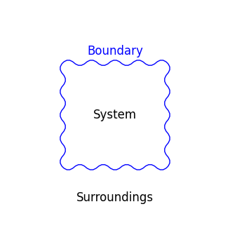
Fig. 12 An isolated system, exchanging neither energy nor matter with its surroundings.

Fundamental Postulate of Statistical Mechanics

Fundamental Postulate

For an isolated system (microcanonical ensemble), each accessible microstate is equally probable.

Hence, the probability of finding the system in the \(i\)-th microstate is:

(12)\[p_i = \frac{1}{M},\]

where \(M\) is the total number of microstates compatible with \(\left( N, V, E \right)\).

Isolated Spin-Up Electron in an f Orbital

Consider an isolated electron with spin up in an \(f\)-orbital. The possible quantum states have magnetic quantum numbers \(m_l = \{-3, -2, -1, 0, 1, 2, 3\}\), giving \(M = 7\). By the fundamental postulate, the probability of each microstate is

\[p_i = \frac{1}{7}.\]