Lecture 2: Essential Python Packages for the Chemical Sciences

One of the key strengths of Python is its extensive ecosystem of packages that cater to various scientific needs, including those in the chemical sciences. These packages extend Python’s capabilities, allowing you to perform complex calculations, analyze data, and visualize results with ease. While there are many packages available, in this lecture, we will focus on some of the most fundamental ones that you’ll be using frequently throughout this course:

• NumPy: The foundation for numerical computing in Python. NumPy provides support for large, multi-dimensional arrays and matrices, along with a collection of mathematical functions to operate on these arrays efficiently.

• SciPy: Built on top of NumPy, SciPy is a library used for scientific and technical computing. It includes modules for optimization, integration, interpolation, eigenvalue problems, and other advanced mathematical tasks.

• Matplotlib: A powerful plotting library that enables you to create a wide variety of static, animated, and interactive visualizations. Matplotlib is particularly useful for generating publication-quality figures in both 2D and 3D.

• Pandas: A versatile library for data manipulation and analysis. Pandas provides data structures like DataFrames, which allow you to work with structured data easily, making tasks such as data cleaning, transformation, and aggregation straightforward.

In this lecture, we will explore the core features of each of these packages, with practical examples to help you understand how they can be applied to solve problems in the chemical sciences.

Learning Objectives

By the end of this lecture, you should be able to:

• Understand the core features and applications of NumPy, SciPy, Matplotlib, and Pandas.

• Perform basic numerical operations and matrix manipulations using NumPy.

• Create and customize plots using Matplotlib.

• Manipulate and analyze data using Pandas DataFrames.

---

Section 1: NumPy - The Foundation of Scientific Computing in Python

NumPy is the cornerstone of scientific computing in Python, providing essential support for large, multi-dimensional arrays and matrices. It also offers a suite of mathematical functions to operate on these arrays, making it indispensable for numerical tasks in the chemical sciences and beyond. Many other scientific libraries, including SciPy, Matplotlib, and Pandas, are built on top of NumPy.

1.1 Key Features of NumPy

• N-dimensional Array Object: NumPy’s array object (ndarray) is a versatile container for data. It can represent vectors, matrices, and higher-dimensional data structures, enabling efficient storage and manipulation of numerical data.

• Broadcasting: Perform element-wise operations on arrays of different shapes in a flexible and efficient manner.

• Linear Algebra, Fourier Transform, and Random Number Generation: NumPy includes a comprehensive suite of functions for these operations, which are critical in many scientific applications.

1.2 Working with NumPy Arrays

Python Lists

A Python list is an ordered collection of items, which can be of any data type. Lists are created using square brackets, e.g., my_list = [1, 2, 3], and are versatile for storing and manipulating sequences of elements. Lists are indexed, meaning each element can be accessed by its position, starting from 0.

NumPy arrays are the core data structure in NumPy. They are similar to Python lists but are more powerful and efficient, particularly for numerical computations. In the chemical sciences, vectors and matrices are ubiquitous, representing quantities such as atomic positions, molecular orientations, and magnetic field components.

Installing NumPy

Before you can start using NumPy, you need to ensure it is installed on your system. You can install NumPy by running the following command in your terminal or command prompt:

pip install numpy

If you’re working within a Jupyter Notebook, you can also install NumPy directly by running:

!pip install numpy

Once NumPy is installed, you’re ready to start creating and working with arrays in Python.

Creating and Using Arrays

Vectors, which play a vital role in representing physical quantities in chemistry, can be created easily with NumPy:

import numpy as np

# Create a 3D vector
v = np.array([1, 2, 3])

# Print the vector
print(v)

# Print the type of v to confirm it's a NumPy array
print(type(v))

[1 2 3]
<class 'numpy.ndarray'>

Matrices are equally important, used to represent systems of equations, Hamiltonians in quantum chemistry, and more. Here’s how you can create a 2x2 matrix:

# Create a 2x2 matrix
M = np.array([[1, 2], [3, 4]])

print(M)

[[1 2]
 [3 4]]

Matrix and Vector Operations

Matrix and vector operations are fundamental in quantum chemistry and many other areas of chemical science. NumPy simplifies these operations:

• Matrix-Vector Multiplication: This operation is common in quantum mechanics, where matrices represent operators and vectors represent states.

Best Practice

Always comment your code to explain the purpose of each section, especially in complex scripts. This makes your code easier to understand and maintain.

# Create a 2x2 matrix
M = np.array([[1, 2], [3, 4]])

# Create a 2D vector
v = np.array([1, 2])

# Multiply the matrix by the vector
w = M @ v

print(w)

[ 5 11]

Reminder

For matrix multiplication, the shape of the resulting array is determined by the shapes of the input arrays. For example, if A has shape (m, n) and B has shape (n, p), then C = A @ B will have shape (m, p).

• Dot Product: The dot product is widely used in quantum chemistry, for example, in verifying the orthonormality of wavefunctions.

# Create two 3D vectors
v = np.array([1, 2, 3])
w = np.array([4, 5, 6])

# Compute the dot product
dot_product = np.dot(v, w)

print(dot_product)

32

Advanced Matrix Operations

In quantum chemistry and other fields, solving linear systems, computing determinants, inverses, and eigenvalues are routine tasks. NumPy makes these operations straightforward:

• Determinant, Inverse, and Eigenvalues:

# Create a 2x2 matrix
M = np.array([[1, 2], [3, 4]])

# Compute the determinant
det = np.linalg.det(M)
print(f"det(M) = {det}")

# Compute the inverse
M_inv = np.linalg.inv(M)
print(f"M_inv = \n{M_inv}")

# Compute the eigenvalues
eigenvalues = np.linalg.eigvals(M)
print(f"eigenvalues = {eigenvalues}")

det(M) = -2.0000000000000004
M_inv = 
[[-2.   1. ]
 [ 1.5 -0.5]]
eigenvalues = [-0.37228132  5.37228132]

Generating Arrays with Specific Properties

NumPy also provides convenient functions for creating arrays with predefined properties, such as arrays filled with zeros, ones, or random numbers:

# Create a 3x3 array of zeros
A = np.zeros((3, 3))
print(A)

# Create a 3x3 array of ones
A = np.ones((3, 3))
print(A)

# Create a 3x3 array of random numbers
A = np.random.rand(3, 3)
print(A)

[[0. 0. 0.]
 [0. 0. 0.]
 [0. 0. 0.]]
[[1. 1. 1.]
 [1. 1. 1.]
 [1. 1. 1.]]
[[0.38848765 0.43260088 0.63391829]
 [0.23067359 0.38986037 0.5963908 ]
 [0.26953356 0.58445442 0.19464139]]

---

1.3 Practice Exercises

1. Exercise 1: Create a 3x3 matrix with random integers between 0 and 9.

   Hint

   Use np.random.randint() to generate random integers.

2. Exercise 2: Create a 3x3 identity matrix.

   Hint

   Use np.eye() to create an identity matrix.

---

Section 2: SciPy - A Powerful Tool for Scientific Computing

While we won’t delve deeply into SciPy in this lecture, it’s a library we’ll return to periodically throughout this course. SciPy builds on the foundation provided by NumPy, offering elegant and efficient solutions for a variety of complex scientific and engineering problems. However, before relying heavily on SciPy, it’s important to understand the underlying principles by building some of these solutions from scratch. Once you have a solid foundation, SciPy will become an invaluable tool in your computational toolkit.

2.1 Key Features of SciPy

• Optimization: SciPy provides robust tools for optimization tasks, such as finding the minimum or maximum of a function. We’ll explore these capabilities in more detail in Lecture 4, where we’ll tackle problems like finding the roots of equations in chemical reaction equilibria.

• Integration: Whether you need to compute definite integrals or solve differential equations, SciPy offers a range of integration techniques. We’ll cover this in Lecture 5, where you’ll learn how to apply these methods to problems such as calculating the overlap integral in chemical bonding.

• Fourier Transforms: Fourier analysis is a critical tool in many scientific fields, including signal processing and spectroscopy. SciPy makes it easy to perform Fourier transforms, enabling you to analyze signals and decompose them into their constituent frequencies.

• And Much More: SciPy is a vast library with modules covering topics like linear algebra, statistics, and image processing. As you progress through this course, you’ll find many opportunities to leverage SciPy’s capabilities. For a full overview of what SciPy offers, you can explore the official documentation.

---

Section 3: Matplotlib - Creating Publication-Quality Visualizations

Matplotlib is a versatile plotting library in Python that allows you to create publication-quality figures across various formats and interactive environments. Whether you need simple plots or complex visualizations, Matplotlib has you covered. With just a few lines of code, you can generate plots, histograms, bar charts, scatterplots, and much more. As a starting point, I highly recommend checking out the “Anatomy of a Figure” graphic from the Matplotlib documentation: Anatomy of a Figure. This reference will be invaluable as we work through different plotting tasks in this course.

3.1 Key Features of Matplotlib

• Wide Range of Plot Types: Create various plots, including line plots, scatter plots, histograms, bar charts, and more.

• Extensive Customization: Customize every aspect of your plots, from colors and line styles to markers and annotations.

• Flexible Output Formats: Save your plots in multiple formats, such as PNG, PDF, and SVG, making it easy to include them in publications, presentations, and reports.

3.2 Creating Basic Plots with Matplotlib

Let’s explore some of the most common plot types you’ll encounter in this course, starting with scatter plots, line plots, and histograms.

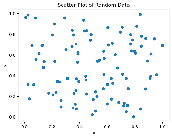
Scatter Plots

Scatter plots are ideal for visualizing relationships between two variables. Here’s how you can create a scatter plot using Matplotlib:

import matplotlib.pyplot as plt
import numpy as np

# Create random data
x = np.random.rand(100)
y = np.random.rand(100)

# Create a scatter plot
plt.scatter(x, y)
plt.xlabel('x')
plt.ylabel('y')
plt.title('Scatter Plot of Random Data')
plt.show()

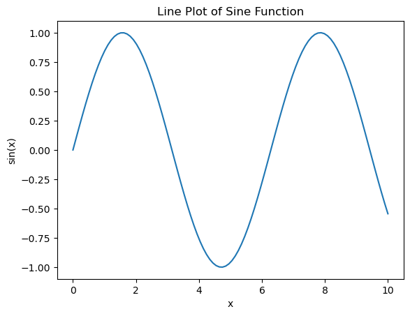
Line Plots

Line plots are commonly used to visualize trends over a range of values. Here’s an example of how to create a simple line plot:

# Create data
x = np.linspace(0, 10, 100)
y = np.sin(x)

# Create a line plot
plt.plot(x, y)
plt.xlabel('x')
plt.ylabel('sin(x)')
plt.title('Line Plot of Sine Function')
plt.show()

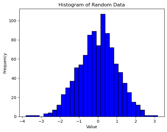
Histograms

Histograms are useful for visualizing the distribution of data. They show how data is spread across different intervals, providing insights into its distribution:

# Create random data
data = np.random.randn(1000)

# Create a histogram
plt.hist(data, bins=30, color='blue', edgecolor='black')
plt.xlabel('Value')
plt.ylabel('Frequency')
plt.title('Histogram of Random Data')
plt.show()

3.3 Customizing Your Plots

One of Matplotlib’s strengths is its ability to customize every aspect of a plot. This includes changing colors, line styles, marker styles, labels, titles, and more. Here’s an example that demonstrates these customization features:

# Create data
x = np.linspace(0, 10, 100)
y = np.sin(x)

# Create a customized line plot
plt.plot(x, y, color='red', linestyle='--', marker='o', label='sin(x)')
plt.xlabel('x')
plt.ylabel('y')
plt.title('Customized Plot of Sine Function')
plt.legend()
plt.grid(True)
plt.show()

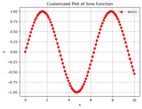
In this example, we’ve customized the plot by changing the line color to red, using a dashed line style, and adding circular markers. We also included a legend, labeled the axes, added a title, and enabled grid lines for better readability.

---

3.4 Practice Exercises

1. Exercise 1: Create a scatter plot of random data with customizations, such as changing the color, marker style, and adding labels.

   Hint

   Use the color and marker parameters in plt.scatter(), and don’t forget to add labels with plt.xlabel() and plt.ylabel().

2. Exercise 2: Create a histogram of random data with customizations, including changing the color, the number of bins, and adding titles and labels.

   Hint

   Use the bins and color parameters in plt.hist() to customize your histogram.

---

Section 4: Pandas - Powerful Data Manipulation in Python

Pandas is like Excel on steroids—think of it as Excel integrated into Python, with far greater flexibility and power. Pandas is a versatile library designed for data manipulation and analysis, providing structures and functions to handle structured data efficiently. It is built on top of NumPy and is particularly useful for working with tabular data, such as spreadsheets and databases.

4.1 Key Features of Pandas

• Flexible Data Structures: Work with labeled data using Pandas’ two primary data structures: Series (1D) and DataFrame (2D). These structures allow you to easily manipulate and analyze data.

• Powerful Data Manipulation: Perform complex operations such as filtering, grouping, merging, and aggregating data with ease.

• Comprehensive I/O Capabilities: Pandas can read and write data in various formats, including CSV, Excel, and SQL databases, making it easy to integrate with other data sources.

4.2 Series: The 1D Data Structure

A Series in Pandas is a one-dimensional labeled array capable of holding any data type, such as integers, strings, or floating-point numbers. You can think of a Series as a single column in an Excel spreadsheet, with an index to label each row.

Here’s how you can create a Series from a NumPy array:

import pandas as pd
import numpy as np

# Create a Series from a NumPy array
s = pd.Series(np.random.randn(5))

print(s)

0    0.302182
1   -1.338002
2    0.673317
3    0.049586
4   -1.656155
dtype: float64

In this Series, the first column represents the index (similar to row numbers in Excel), and the second column holds the data.

Important

By default, Python uses zero-based indexing, so the first element in a NumPy array or Pandas DataFrame has an index of 0.

4.3 DataFrame: The 2D Data Structure

A DataFrame is a two-dimensional labeled data structure, similar to an Excel spreadsheet, where each column can contain different data types. DataFrames are the bread and butter of data manipulation in Pandas, allowing you to organize and manipulate data in powerful ways.

Here’s how to create a DataFrame from a dictionary of NumPy arrays:

# Create a DataFrame from a dictionary of NumPy arrays
data = {
    'A': np.random.randn(5),
    'B': np.random.rand(5)
}

df = pd.DataFrame(data)

print(df)

          A         B
0  2.192456  0.405787
1  0.826182  0.320524
2 -0.038889  0.840733
3 -0.066214  0.089069
4 -1.534060  0.328712

In this DataFrame, the index column functions like the row numbers in Excel, and each key in the dictionary becomes a column. The DataFrame provides the power to manipulate and analyze your data more efficiently than traditional spreadsheet software.

4.4 Reading and Writing Data

Pandas provides functions for reading and writing data in a variety of formats, such as CSV, Excel, and SQL databases. For this example, you can download the data.csv file we’ll be using here.

# Read data from a CSV file
df = pd.read_csv('data.csv')

print(df)

      Element  Per Mole  Per Atom Per Mole Unit Per Atom Unit
0    Actinium    410.00      4.25        kJ/mol       eV/atom
1    Aluminum    327.00      3.39        kJ/mol       eV/atom
2   Americium    264.00      2.73        kJ/mol       eV/atom
3    Antimony    265.00      2.75        kJ/mol       eV/atom
4       Argon      7.74      0.08        kJ/mol       eV/atom
..        ...       ...       ...           ...           ...
85      Xenon     15.90      0.16        kJ/mol       eV/atom
86  Ytterbium    154.00      1.60        kJ/mol       eV/atom
87    Yttrium    422.00      4.37        kJ/mol       eV/atom
88       Zinc    130.00      1.35        kJ/mol       eV/atom
89  Zirconium    603.00      6.25        kJ/mol       eV/atom

[90 rows x 5 columns]

This dataset includes information like element names and their cohesive energies (the energy required to separate atoms in a solid to infinite distances), stored in units of kJ/mol and eV/atom. Pandas also allows you to write this data to a CSV file using the to_csv method:

# Write the DataFrame to a CSV file
df.to_csv('output.csv', index=False)

Setting index=False prevents the index from being written to the file, which is useful if you want a clean output.

4.5 Filtering Data

One of Pandas’ strengths is its ability to filter data based on conditions. For example, you can filter a DataFrame to display only the rows where the cohesive energy falls within a specific range:

Note

The & operator is used for element-wise logical AND operations in Pandas. You can also use | for OR operations, ~ for NOT operations, == for equality, and parentheses for grouping conditions.

# Filter rows where the cohesive energy is between 50 and 100 kJ/mol
filtered_df = df[(df['Per Mole'] > 50) & (df['Per Mole'] < 100)]

print(filtered_df)

      Element  Per Mole  Per Atom Per Mole Unit Per Atom Unit
15     Cesium      77.6     0.804        kJ/mol       eV/atom
24   Fluorine      81.0     0.840        kJ/mol       eV/atom
42    Mercury      65.0     0.670        kJ/mol       eV/atom
57  Potassium      90.1     0.934        kJ/mol       eV/atom
63   Rubidium      82.2     0.852        kJ/mol       eV/atom

This filtering technique is incredibly useful when working with large datasets, allowing you to focus on subsets of data that meet specific criteria.

---

4.6 Practice Exercises

1. Exercise 1: Create a DataFrame from a dictionary of NumPy arrays and write it to a CSV file.

   Hint

   Use the pd.DataFrame() function to create the DataFrame, and to_csv() to save it to a file.

2. Exercise 2: Read data from a CSV file into a DataFrame, then filter the data based on a condition.

   Hint

   Use pd.read_csv() to load the data and the filtering syntax shown above to filter the DataFrame.

3. Exercise 3: Filter a DataFrame based on a different condition. For example, try filtering for rows where the cohesive energy is greater than 150 kJ/mol.

   Hint

   Modify the filtering condition in the example provided.

---

This concludes our second lecture. As you practice using these essential Python packages, you’ll gain confidence in applying them to solve complex problems in the chemical sciences. The skills you develop here will serve as a strong foundation for your computational work, both in this course and beyond.