Finding descriptors for catalysis using random forests
In this tutorial, I’m going to show you how easy it is to train and analyze a random forest regression model. The data we’re going to use is taken from my recent paper on tuning the hydrogen evolving activity of Ni2P via strain. [1] The main idea of the paper is that surface nonmetal dopants, which replace P near the Ni3 sites, can induce compressive and tensile strain on the Ni3 sites leading to changes in their H binding strength.
In my study, I calculated the H binding energy at the Ni3 site for different nonmetal dopants (B, C, N, O, Si, S, As, Se, & Te) and doping concentrations. There were 55 configurations in total…so I was working with a rather small data set. I should mention that for smaller data sets it’s generally advisable to use linear models, however, if care is taken, then random forests can be used as well. Regardless, always make sure to validate your proposed descriptors using an appropriate simulation technique such as density functional theory.
A quick word on random forests. Random forests are made up of decision trees. Each decision tree gets a random subset of the rows and columns of the data and is built using the CART algorithm. [2] For more information, please see chapter 2.4 of my thesis.
[1] Wexler, R. B.; Martirez, J. M. P.; Rappe, A. M. Chemical Pressure-Driven Enhancement of the Hydrogen Evolving Activity of Ni2P from Nonmetal Surface Doping Interpreted via Machine Learning. J. Am. Chem. Soc. 2018, 140 (13), pp 4678-4683. DOI: 10.1021/jacs.8b00947
[2] L. Breiman, J. Friedman, R. Olshen, and C. Stone. Classification and Regression Trees. Wadsworth, Belmont, CA, 1984.*
# import necessary modules
import numpy as np
import pandas as pd
import matplotlib.pyplot as plt
from sklearn.model_selection import train_test_split
from sklearn.ensemble import RandomForestRegressor
from sklearn.metrics import r2_score
from sklearn.metrics import mean_squared_error
from sklearn.metrics import mean_absolute_error
numpy and pandas are used for convenient data storage, matplotlib is used to generate plots, and the scikit learn is used for all things machine learning. For example, we use train_test_split to do as its name suggests, RandomForestRegressor trains a random forest, and r2_score, mean_squared_error, and mean_absolute_error are different evaluation metrics (you may like one of them more than the others, though MSE is probably the most robust).
# helper functions
def drop_nzv(df, min_var = 0.05) :
    """ drop near zero variance descriptors
    note: y should be your last column
    """
    to_drop = list()
    for i in range(df.shape[1] - 1) :
        descriptor = df.columns[i]
        data_type = df.dtypes[i]
        if (data_type == "int64") | (data_type == "float64") :
            variance = df.iloc[:, i].var()
            if variance <= min_var :
                to_drop.append(descriptor)
    to_drop = np.array(to_drop)
    return df.drop(to_drop, axis = 1)

def get_results(model, X, y) :
    r2 = r2_score(y, model.predict(X))
    rmse = np.sqrt(mean_squared_error(y, model.predict(X)))
    mae = mean_absolute_error(y, model.predict(X))
    return r2, rmse, mae

def plot_results(model, X_train, X_test, y_train, y_test, X_val = np.array([]), y_val = np.array([]), data_range = [-0.5, 0.5]) :
    plt.scatter(y_train, model.predict(X_train), color = "blue", alpha = 0.5)
    plt.scatter(y_test, model.predict(X_test), color = "red", alpha = 0.5)
    if X_val.size != 0 :
        plt.scatter(y_val, model.predict(X_val), color = "green")
    plt.plot(data_range, data_range, color = "black")
    plt.xlabel("DFT")
    plt.ylabel("Predicted")
    plt.show()

def plot_importances(model, descriptors) :
    plt.bar(np.arange(model.feature_importances_.shape[0]), model.feature_importances_)
    plt.xticks(np.arange(model.feature_importances_.shape[0]), descriptors, rotation=90$$)
    plt.show()
This chunk contains some functions that you may find useful. drop_nzv takes a dataframe and removes columns whose variance is small, i.e. they are nearly single valued and therefore cannot be used to describe variations in \(y\). get_results takes a model and calculates the three performance metrics mentioned above. plot_results plots the actual \(y\) vs. the prediction for both the training and test set.
At this point, we’re ready to start writing some real code. You can download the data from my paper at HERE.
# read and inspect data
df = pd.read_csv("/Users/rwexler/Downloads/Machine_Learning/processed_data.csv")
print(df.shape)
df.head()
(55, 31)
| Unnamed: 0 | X | nX | X95_98 | X95_100 | X98_100 | X98_95_100 | X95_98_100 | X95_100_98 | Avg_Ni_Ni | ... | q106_5 | q107_6 | Z | m | r | Avg_qNi | Std_qNi | Avg_qX | Std_qX | dGH | |
|---|---|---|---|---|---|---|---|---|---|---|---|---|---|---|---|---|---|---|---|---|---|
| 0 | 1 | As | 1 | 2.772373 | 2.728643 | 2.673381 | 58.146831 | 60.107425 | 61.745744 | 2.724799 | ... | -999.0000 | -999.0 | 33 | 74.92 | 121 | 0.632433 | 0.016967 | -0.370600 | -999.000000 | -0.467393 |
| 1 | 3 | As | 2 | 2.701154 | 2.593942 | 2.637543 | 59.709237 | 58.125061 | 62.165703 | 2.644213 | ... | -999.0000 | -999.0 | 33 | 74.92 | 121 | 0.627867 | 0.015033 | -0.404850 | 0.024537 | -0.480859 |
| 2 | 5 | As | 3 | 2.682490 | 2.685299 | 2.680348 | 59.912592 | 60.095729 | 59.991680 | 2.682712 | ... | -999.0000 | -999.0 | 33 | 74.92 | 121 | 0.619267 | 0.003819 | -0.415900 | 0.004303 | -0.352070 |
| 3 | 7 | As | 4 | 2.644063 | 2.569793 | 2.657188 | 61.260029 | 57.991838 | 60.748134 | 2.623681 | ... | -999.0000 | -999.0 | 33 | 74.92 | 121 | 0.604533 | 0.026364 | -0.409075 | 0.014458 | -0.410929 |
| 4 | 9 | As | 5 | 2.675141 | 2.611050 | 2.575125 | 58.290699 | 59.609085 | 62.100216 | 2.620439 | ... | -0.3967 | -999.0 | 33 | 74.92 | 121 | 0.589967 | 0.025755 | -0.405520 | 0.014240 | -0.441036 |
5 rows × 31 columns
As you can see, there are 55 rows and 31 columns. Information about each of the columns can be found in processed_data.txt, which comes along with the data. Suffice to say, there are some structure (bond length, angle, etc.) and charge (Lowdin charges) descriptors for each surface and it’s corresponding H binding energy at the Ni3 site (\(\Delta G_{\rm H}\)) calculated using DFT with the GGA of PBE for the electron exchange and correlation and using DFT-D2 vdW corrections. If this terminology seems foreign to you, I recommend reading chapter 2.1 of my thesis. The first column is useless and can be removed as follows:
# drop first column
df = df.drop(["Unnamed: 0"], axis = 1)
df.head()
| X | nX | X95_98 | X95_100 | X98_100 | X98_95_100 | X95_98_100 | X95_100_98 | Avg_Ni_Ni | Std_Ni_Ni | ... | q106_5 | q107_6 | Z | m | r | Avg_qNi | Std_qNi | Avg_qX | Std_qX | dGH | |
|---|---|---|---|---|---|---|---|---|---|---|---|---|---|---|---|---|---|---|---|---|---|
| 0 | As | 1 | 2.772373 | 2.728643 | 2.673381 | 58.146831 | 60.107425 | 61.745744 | 2.724799 | 0.049608 | ... | -999.0000 | -999.0 | 33 | 74.92 | 121 | 0.632433 | 0.016967 | -0.370600 | -999.000000 | -0.467393 |
| 1 | As | 2 | 2.701154 | 2.593942 | 2.637543 | 59.709237 | 58.125061 | 62.165703 | 2.644213 | 0.053916 | ... | -999.0000 | -999.0 | 33 | 74.92 | 121 | 0.627867 | 0.015033 | -0.404850 | 0.024537 | -0.480859 |
| 2 | As | 3 | 2.682490 | 2.685299 | 2.680348 | 59.912592 | 60.095729 | 59.991680 | 2.682712 | 0.002483 | ... | -999.0000 | -999.0 | 33 | 74.92 | 121 | 0.619267 | 0.003819 | -0.415900 | 0.004303 | -0.352070 |
| 3 | As | 4 | 2.644063 | 2.569793 | 2.657188 | 61.260029 | 57.991838 | 60.748134 | 2.623681 | 0.047128 | ... | -999.0000 | -999.0 | 33 | 74.92 | 121 | 0.604533 | 0.026364 | -0.409075 | 0.014458 | -0.410929 |
| 4 | As | 5 | 2.675141 | 2.611050 | 2.575125 | 58.290699 | 59.609085 | 62.100216 | 2.620439 | 0.050665 | ... | -0.3967 | -999.0 | 33 | 74.92 | 121 | 0.589967 | 0.025755 | -0.405520 | 0.014240 | -0.441036 |
5 rows × 30 columns
Viola! Now, let’s use our drop_nzv function to remove descriptors that have no predictive capability.
# drop near zero variance descriptors
df = drop_nzv(df)
df.head()
| X | nX | X95_98 | X95_100 | X98_100 | X98_95_100 | X95_98_100 | X95_100_98 | Avg_Ni_Ni | Std_Ni_Ni_Ni | ... | q105_3 | q108_4 | q106_5 | q107_6 | Z | m | r | Avg_qX | Std_qX | dGH | |
|---|---|---|---|---|---|---|---|---|---|---|---|---|---|---|---|---|---|---|---|---|---|
| 0 | As | 1 | 2.772373 | 2.728643 | 2.673381 | 58.146831 | 60.107425 | 61.745744 | 2.724799 | 1.801860 | ... | -999.0000 | -999.0000 | -999.0000 | -999.0 | 33 | 74.92 | 121 | -0.370600 | -999.000000 | -0.467393 |
| 1 | As | 2 | 2.701154 | 2.593942 | 2.637543 | 59.709237 | 58.125061 | 62.165703 | 2.644213 | 2.035953 | ... | -999.0000 | -999.0000 | -999.0000 | -999.0 | 33 | 74.92 | 121 | -0.404850 | 0.024537 | -0.480859 |
| 2 | As | 3 | 2.682490 | 2.685299 | 2.680348 | 59.912592 | 60.095729 | 59.991680 | 2.682712 | 0.091852 | ... | -0.4203 | -999.0000 | -999.0000 | -999.0 | 33 | 74.92 | 121 | -0.415900 | 0.004303 | -0.352070 |
| 3 | As | 4 | 2.644063 | 2.569793 | 2.657188 | 61.260029 | 57.991838 | 60.748134 | 2.623681 | 1.757853 | ... | -0.4179 | -0.3876 | -999.0000 | -999.0 | 33 | 74.92 | 121 | -0.409075 | 0.014458 | -0.410929 |
| 4 | As | 5 | 2.675141 | 2.611050 | 2.575125 | 58.290699 | 59.609085 | 62.100216 | 2.620439 | 1.934610 | ... | -0.4162 | -0.3846 | -0.3967 | -999.0 | 33 | 74.92 | 121 | -0.405520 | 0.014240 | -0.441036 |
5 rows × 24 columns
As a final preprocessing step, we’ll want to remove descriptors that are highly correlated. The reason we may want to do this is because linearly dependent descriptors are redundant, i.e. only one is necessary to explain their affect on \(y\), and models with fewer descriptors are often preferred, especially in the physical sciences! As such, I’ll remove descriptors that have correlation coefficients greater than 0.95. This chunk was adapted from an awesome blog post by Chris Albon.
# drop highly correlated descriptors
corr_matrix = df.iloc[:, :-1].corr().abs()
upper = corr_matrix.where(np.triu(np.ones(corr_matrix.shape), k=1).astype(np.bool))
to_drop = [column for column in upper.columns if any(upper[column] > 0.95)]
df = df.drop(to_drop, axis = 1)
print(df.shape)
df.head()
(55, 18)
| X | nX | X95_98 | X95_100 | X98_100 | X98_95_100 | X95_98_100 | X95_100_98 | Std_Ni_Ni_Ni | q104_1 | q103_2 | q105_3 | q108_4 | q106_5 | q107_6 | Z | r | dGH | |
|---|---|---|---|---|---|---|---|---|---|---|---|---|---|---|---|---|---|---|
| 0 | As | 1 | 2.772373 | 2.728643 | 2.673381 | 58.146831 | 60.107425 | 61.745744 | 1.801860 | -0.3706 | -999.0000 | -999.0000 | -999.0000 | -999.0000 | -999.0 | 33 | 121 | -0.467393 |
| 1 | As | 2 | 2.701154 | 2.593942 | 2.637543 | 59.709237 | 58.125061 | 62.165703 | 2.035953 | -0.3875 | -0.4222 | -999.0000 | -999.0000 | -999.0000 | -999.0 | 33 | 121 | -0.480859 |
| 2 | As | 3 | 2.682490 | 2.685299 | 2.680348 | 59.912592 | 60.095729 | 59.991680 | 0.091852 | -0.4117 | -0.4157 | -0.4203 | -999.0000 | -999.0000 | -999.0 | 33 | 121 | -0.352070 |
| 3 | As | 4 | 2.644063 | 2.569793 | 2.657188 | 61.260029 | 57.991838 | 60.748134 | 1.757853 | -0.4174 | -0.4134 | -0.4179 | -0.3876 | -999.0000 | -999.0 | 33 | 121 | -0.410929 |
| 4 | As | 5 | 2.675141 | 2.611050 | 2.575125 | 58.290699 | 59.609085 | 62.100216 | 1.934610 | -0.4151 | -0.4150 | -0.4162 | -0.3846 | -0.3967 | -999.0 | 33 | 121 | -0.441036 |
After having cleaned up our data set, we’re now left with only 17 descriptors and 1 column for \(y\) at the far right.
A critical step in the construction of machine learning models is splitting the data into a training and test set. The training set is used to build the model whereas the test set is kept aside, not analyzed, and used only for evaluating the “out of sample” error. The splitting should be done randomly, however, there are some more advanced schemes, e.g. those that split the data so that the distribution of \(y\) values in each subset is more or less the same. Here, we’ll just randomly split the data. Often a good starting point is to use 2/3 of the data for training and 1/3 for testing, however, this is not a hard and fast rule and probably leans towards “too conservative”.
# split training and testing set
X = df.iloc[:, 1:-1]
y = df.dGH
X_train, X_test, y_train, y_test = train_test_split(X, y, test_size=0.33, random_state=42)
Tune random forest
n_estimators
Random forests have a few parameters that we’ll need to tune in order to minimize the test set error. The first is the number of trees in the random forests, a.k.a. n_estimators, which we’ll vary from 1 to 40.
# tune n_estimators
n_estimators_list = np.arange(1, 41, 1)
r2_train = np.zeros(n_estimators_list.shape)
r2_test = np.zeros(n_estimators_list.shape)
for i, n_estimators in enumerate(n_estimators_list) :
    regr_2 = RandomForestRegressor(n_estimators=n_estimators, random_state=42)
    regr_2.fit(X_train, y_train)
    r2_train[i] = get_results(regr_2, X_train, y_train)[0]
    r2_test[i] = get_results(regr_2, X_test, y_test)[0]
plt.plot(n_estimators_list, r2_train, color = "blue")
plt.plot(n_estimators_list, r2_test, color = "red")
plt.xlabel("n estimators")
plt.ylabel(r"R$^2$")
plt.grid(True)
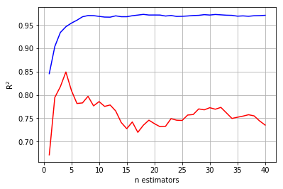
The blue and red lines are the training and test set error, respectively. Tuning n_estimators ultimately boils down to choosing the value that minimizes test set error, or in the case of the plot above, maximizes \(R^{2}\). Therefore, our tuning indicates that a small random forest with 4 trees is best.
max_features
Next, we’ll tune the number of features available to each tree during it’s training, a.k.a. max_features, from 1 (an overly simple and rather silly model unless that one descriptor rocks) to the total number of descriptors that survived our preprocessing above (17).
# max_features
max_features_list = np.arange(1, X_train.shape[1] + 1)
r2_train = np.zeros(max_features_list.shape)
r2_test = np.zeros(max_features_list.shape)
for i, max_features in enumerate(max_features_list) :
    regr_2 = RandomForestRegressor(max_features=max_features, random_state=42, n_estimators=4)
    regr_2.fit(X_train, y_train)
    r2_train[i] = get_results(regr_2, X_train, y_train)[0]
    r2_test[i] = get_results(regr_2, X_test, y_test)[0]
plt.plot(max_features_list, r2_train, color = "blue")
plt.plot(max_features_list, r2_test, color = "red")
plt.xlabel("max features")
plt.ylabel(r"R$^2$")
plt.grid(True)
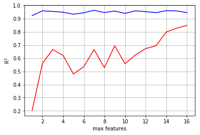
Here you can see that the best model includes all of the descriptors.
max_depth
Finally, we may want to tune the maximum depth of the trees, a.k.a. max_depth, from 1 to some arbitrarily large number, e.g. 31.
# max_depth
max_depths = np.arange(1, 31, 1)
r2_train = np.zeros(max_depths.shape)
r2_test = np.zeros(max_depths.shape)
for i, max_depth in enumerate(max_depths) :
    regr_2 = RandomForestRegressor(max_depth=max_depth, random_state=42, n_estimators=4, max_features=16)
    regr_2.fit(X_train, y_train)
    r2_train[i] = get_results(regr_2, X_train, y_train)[0]
    r2_test[i] = get_results(regr_2, X_test, y_test)[0]
plt.plot(max_depths, r2_train, color = "blue")
plt.plot(max_depths, r2_test, color = "red")
plt.xlabel("max depth")
plt.ylabel(r"R$^2$")
plt.grid(True)
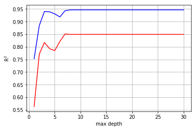
It’s clear that deeper trees are better, however, after 7 layers, depth does’nt improve the model and can only lead to overfitting. As such, we’ll stick with a model with 4 trees, 16 descriptors, and a maximum depth of 7 layers.
Now we’re ready to train our random forest regressor!
# train random forest
regr = RandomForestRegressor(n_estimators = 4,
max_features = 16,
max_depth = 7,
random_state=42)
regr.fit(X_train, y_train)
# print results
r2, rmse, mae = get_results(regr, X_test, y_test)
print("results")
print("-------")
print("r2 =", r2)
print("rmse =", rmse)
print("mae =", mae)
# plot results
plot_results(regr, X_train, X_test, y_train, y_test)
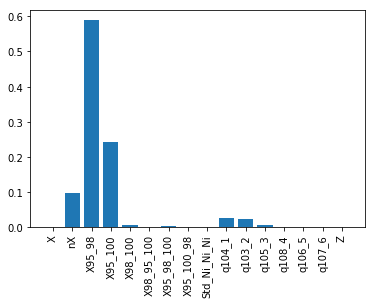
# plot descriptor importances
plot_importances(regr, df.columns[:-1])
results
-------
r2   = 0.8510929000114282
rmse = 0.07531117819235955
mae  = 0.0525640930241579
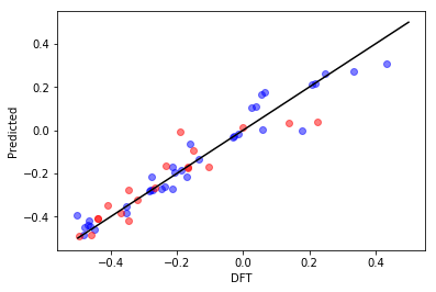
All righty, then! Let’s take this piece by piece. First, your \(R^{2}\) is 0.85, which is pretty darn good considering we only fed the model simple structure and charge descriptors. The RMSE and MAE are between 0.05 and 0.1 eV, which is excellent considering the intrinsic DFT accuracy for binding energies is around 0.1 eV. The first plot shows how well our random forest model did compared to DFT. The black line shows perfect performance. The blue and red dots correspond to the training and test data, respectively. Upon visual inspection and in conjuction with the metrics above, we have achieved a good fit.
Finally, because random forests are intrinsically nonlinear models, they aren’t as interpretable as, say, multiple linear regression models. However, we can look under the hood of the random forest model to see which descriptors were the most effective in making these predictions. Simply put, the most important features are those that reduce the training set error the most. There are various ways of calculating this reduction but their description is beyond the scope of this introduction.
So what does the bottom plot tell us? It tells us that the most important descriptor, i.e. the one with the largest bar, is for X95_98, which is the bond distance between two Ni’s at the Ni3 site. This means that Ni-Ni bond distance is the most important descriptor of H binding strength. Since we kept the active site the same (Ni3) and applied chemical perturbations around it (replacing P with other nonmetals), our random forest model suggests that dopants simply apply strain on the Ni3 site, modulating its H binding strength via compression and expansion.
The end
I hope you enjoyed this introduction. Please feel free to get in touch if you have any questions/comments about this and/or suggestions for future content! And, as always, thanks for using this resource!