Course Introduction

1. Course Introduction#

1.1. Overview#

This course covers the fundamental concepts of thermodynamics and statistical mechanics, along with their applications to chemical systems. It builds upon the thermodynamic principles introduced in Chem 106 and Chem 112, and the quantum mechanics taught in Chem 105, Chem 111, and Chem 401. By connecting molecular-level behavior to macroscopic thermodynamic observations, students will learn how theory underpins real-world chemical processes.

1.2. Why Study Thermodynamics and Statistical Mechanics?#

1.2.1. Bridging the Microscopic and Macroscopic Worlds#

Typical chemical systems contain on the order of Avogadro’s number of particles (i.e., \(N_\text{A} = 6.022 \times 10^{23}\)). Thermodynamics abstracts the complexity of such large collections of molecules into a framework for predicting:

Reaction spontaneity,
Equilibrium states,
Phase transitions, and more.

1.2.2. Modern Applications#

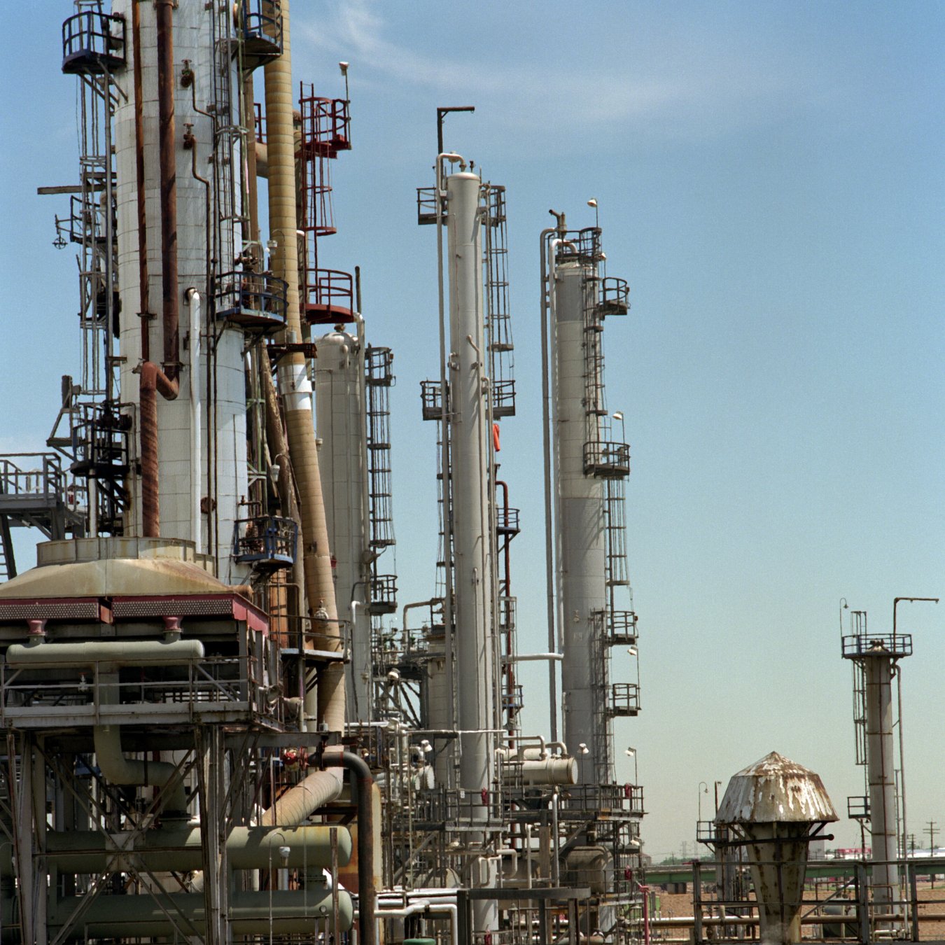
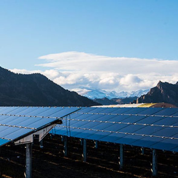
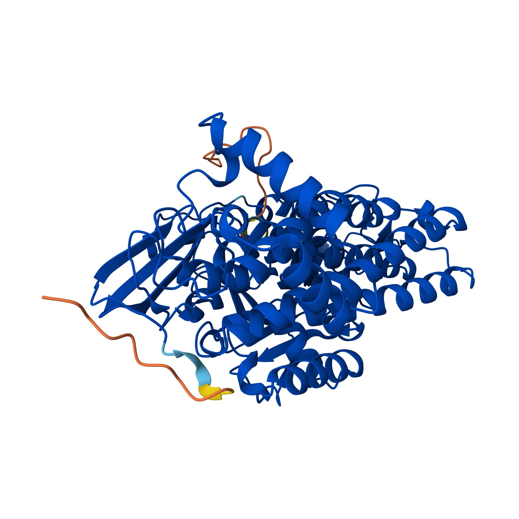
Thermodynamics and statistical mechanics are central to diverse fields, including industrial chemistry, materials science, and biochemistry. The examples below highlight just a few applications:

Industrial Chemistry

Predicting reaction spontaneity and modeling large-scale chemical processes.

Materials Chemistry

Designing advanced materials for optical, electronic, or mechanical applications.

Biochemistry

Investigating protein folding and enzyme activity in biological systems.

1.3. Key Definitions#

1.3.1. Thermodynamic Systems#

_images/16c10b90c7dafb3c4de8357fa528894f6e9199381989b3db45760d51dd591c81.png — Fig. 1.4 **Types of thermodynamic systems:** (a) **Isolated**—no exchange of energy or matter; (b) **Closed**—exchanges energy but not matter; and (c) **Open**—exchanges both energy and matter.#

System#: The portion of the universe chosen for study, separated from its surroundings by a boundary.
Surroundings#: Everything external to the system that can exchange energy or matter with it.
Boundary#: The interface separating a system from its surroundings.
Isolated system#: Exchanges neither energy nor matter with its surroundings.
Closed system#: Exchanges energy but not matter with its surroundings.
Open system#: Exchanges both energy and matter with its surroundings.

1.3.2. State of a System#

        ---
config:
  flowchart:
    htmlLabels: false
  layout: elk
  look: handDrawn
  theme: neutral

---
flowchart TB
  subgraph B["Microscopic"]
    direction TB
      B1["Classical"] ~~~ B2["Quantum"]
  end

  subgraph C["Macroscopic"]
    direction TB
      C1["Equilibrium"]
  end

  subgraph C1["Equilibrium"]
    direction TB
      C11["Thermodynamic"]
  end

  subgraph C11["Thermodynamic"]
    direction LR
      C111["State variables"] ~~~ C112["State functions"] & C113["Path functions"]
  end

  subgraph C111["State variables"]
    direction TB
      C1111["Extensive"] ~~~ C1112["Intensive"]
  end

  A["State of a system"] --> B & C

Particle#: A microscopic entity such as an atom, molecule, or ion.
Microscopic state (classical)#: Positions and momenta of all particles in the system.
Microscopic state (quantum)#: The wavefunction describing the system’s particles.
Equilibrium#: A condition in which macroscopic properties remain constant over time.
Thermodynamic equilibrium#: A state of simultaneous mechanical, thermal, and chemical equilibrium.
Thermodynamic state#: A set of macroscopic variables defining a system in equilibrium.
State variable#: A property that defines a system’s state.
State function#: A property depending only on the system’s state, not on the path taken.
Equation of state#: A mathematical relationship among state variables.
Path function#: A property depending on the process or path taken between states.
Process#: A transformation changing a system from one state to another.
Extensive property#: A property proportional to system size (e.g., volume, entropy).
Intensive property#: A property independent of system size (e.g., temperature, pressure).

1.4. Basic Forms of Energy and Energy Transfer#

        ---
config:
  flowchart:
    htmlLabels: false
  layout: elk
  look: handDrawn
  theme: neutral

---
flowchart TB
  subgraph H1["Electrostatic"]
    direction TB
      H11["Charge–charge"] ~~~ H12["Charge–dipole"]
  end
  subgraph H2["van der Waals"]
    direction TB
      H21["Dipole–dipole"] ~~~ H22["Induced dipole"] ~~~ H23["Dispersion"]
  end
  subgraph H["Electric"]
    direction LR
      H1 ~~~ H2
  end
  subgraph I1["Intramolecular"]
    direction TB
      I11["Covalent"] ~~~ I12["Ionic"] ~~~ I13["Metallic"]
  end
  subgraph I2["Intermolecular"]
    direction TB
      I21["Hydrogen"] ~~~ I22["van der Waals"]
  end
  subgraph I["Chemical"]
    direction LR
      I1 ~~~ I2
  end
  subgraph J["Mechanical"]
    direction TB
      J1["Expansion"] ~~~ J2["Surface expansion"] ~~~ J3["Extension"]
  end
  subgraph G["Work"]
    direction LR
      J ~~~ G1["Electrical"]
  end

  A["Basic forms of energy and energy transfer"] --> B["Energy"] & C["Energy transfer"]
  B --> D["Kinetic"] & E["Potential"]
  C --> F["Heat"] & G
  E --> H & I
  H1 & H2
  I1 & I2

  style H11 stroke:red, stroke-width:2px
  style H2 stroke:blue, stroke-width:2px
  style I12 stroke:red, stroke-width:2px
  style I22 stroke:blue, stroke-width:2px

1.4.1. Energy#

Kinetic energy#: Energy due to motion (e.g., a moving particle).
Potential energy#: Energy due to position or configuration (e.g., a stretched spring).
Internal energy#: The total microscopic kinetic and potential energy of a system, averaged over its microstates.

1.4.2. Energy Transfer#

Work#: Energy transferred when a force acts over a distance (e.g., lifting a mass).
Heat#: Energy transferred because of a temperature difference (e.g., conduction from hot to cold).

1.5. Important Units#

1.5.1. SI Units#

Table 1.1 **Base SI Units**#
Quantity	Unit	Symbol
Time	second	s
Length	meter	m
Mass	kilogram	kg
Temperature	kelvin	K

[4]

Table 1.2 **Derived SI Units**#
Quantity	Unit	Symbol	Conversion
Frequency	hertz	Hz	\(1 \,\text{Hz} = 1 \,\text{s}^{-1}\)
Force	newton	N	\(1 \,\text{N} = 1 \,\text{kg m s}^{-2}\)
Pressure	pascal	Pa	\(1 \,\text{Pa} = 1 \,\text{N m}^{-2}\)
Energy	joule	J	\(1 \,\text{J} = 1 \,\text{N m}\)

1.5.2. Non-SI Units#

Table 1.3 **Non-SI Units**#
Quantity	Unit	Symbol	Conversion
Pressure	bar	bar	\(1 \,\text{bar} = 1 \times 10^5 \,\text{Pa}\)
	atmosphere	atm	\(1 \,\text{atm} \approx 1.01325 \,\text{bar}\)
	torr	torr	\(1 \,\text{torr} = \frac{1}{760}\,\text{atm}\)
	millimeters of mercury	mmHg	\(1 \,\text{mmHg} = 1 \,\text{torr}\)
Energy	electronvolt	eV	\(1 \,\text{eV} = 1.602 \times 10^{-19} \,\text{J}\)
	calorie	cal	\(1 \,\text{cal} = 4.184 \,\text{J}\)

[5] [6] [7]