Introduction to the Atomic Simulation Environment
The Atomic Simulation Environment (ASE) is a set of useful Python modules for manipulating and visualizing structures, setting up calculations/simulations, and converting between different file formats. Here is a link to ASE’s documentation: https://wiki.fysik.dtu.dk/ase/
Some things that you can do with ASE are as follows:
- Visualize structures
- Set up and run DFT/PAW calculations using VASP
- Perform structure optimization using a wide range of algorithms, e.g. BFGS
- Automate ENCUT and KPOINTS convergence tests
Contents
Installation
ASE can be installed using pip as follows:
pip install --user ase
Then you can import ASE just like any other Python module.
Working Examples
For the following working examples, I will first present the code block, then explain it line-by-line (for the most part), and finally show the result.
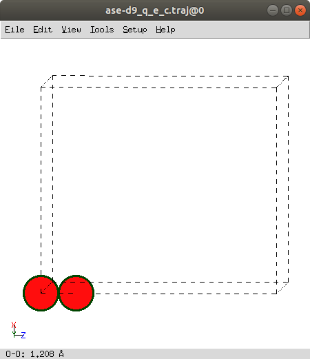
Visualizing the O2 Dimer in a Box
from ase import Atoms, Atom
from ase.visualize import view

d = 1.208
o2 = Atoms([Atom("O", [0, 0, 0]),
	    Atom("O", [0, 0, d])],
           cell = [(7, 0, 0),
                   (0, 7.5, 0),
                   (0, 0, 8)])
o2.set_pbc((True, True, True))
view(o2)
The first two lines import the ASE modules we will need to generate and visualize the O2 dimer. An “Atom” object contains information about a particular atom, e.g. element symbol and position. An “Atoms” object contains information about the whole system, which in this case is two O atoms separated by 1.208 Å. Finally, the “view” function takes an “Atoms” object as an argument and opens the ASE GUI, which shows an interactive 3D rendering of the system. If you Ctrl click on both atoms, then the dialog box at the bottom of the GUI will print the bond distance.
Calculating the Total Energy of the O2 Dimer Using VASP
Before you can run VASP using ASE, you have to tell ASE where the VASP executable and PAW potentials are located. ASE recommends that you create a directory called vasp in $HOME. In $HOME/vasp, create a file called run_vasp.py with the following contents:
import os
exitcode = os.system('$VASP_EXEC')
#exitcode = os.system('srun -n 40 $VASP_EXEC > log')
The first line imports a package called os that enables the use of shell commands in Python. The second line calls the VASP executable, which is globally defined as $VASP_EXEC on my computer. The third line, which is commented out, enables parallel execution of VASP over 40 cores using srun and writes the standard output to a file called log. This script needs to be modified if you want to change the number of cores. Next, ASE recommends that you create another directory inside $HOME/vasp called mypps where the PAW potentials will be stored. Inside $HOME/vasp/mypps there should be three subdirectories called potpaw, potpaw_GGA, and potpaw_PBE. The first and last contain LDA and GGA-PBE PAW potentials, respectively. You can leave potpaw_GGA empty. Finally, add the following to your .bashrc file so that ASE can find $HOME/vasp and its contents:
export VASP_SCRIPT=$HOME/vasp/run_vasp.py
export VASP_PP_PATH=$HOME/vasp/mypps
Now you are ready to run VASP using ASE.
from ase import Atoms, Atom
from ase.calculators.vasp import Vasp

d = 1.208
o2 = Atoms([Atom("O", [0, 0, 0], magmom = 1),
            Atom("O", [0, 0, d], magmom = 1)],
           cell = [(7, 0, 0),
                   (0, 7.5, 0),	Edit
                   (0, 0, 8)])
o2.set_pbc((True, True, True))

calc = Vasp(prec = "Accurate",
            ediff = 1E-5,
            xc = "pbe",
            gamma = True)
o2.set_calculator(calc)
total_energy = o2.get_potential_energy()
print(total_energy)
The first ten lines are the same as the previous example with the exception that, on line 2, the Vasp calculator is imported from ase.calculators.vasp. The calculator is defined on line 12 and, for the most part, the calculator’s arguments are lower case versions of INCAR tags (https://cms.mpi.univie.ac.at/wiki/index.php/Category:INCAR). The only argument that is not an INCAR tag is gamma, which is True for Γ-point calculations and False otherwise. In lines 16 and 17, the VASP calculator calc is attached to the o2 object and the get_potential_energy method is called, running a VASP single-point calculation of the total energy. The final line prints the total energy, which is -9.81923384 eV (note: exact value depends on the PAW potentials).
Optimizing the Bond Length of O2 Dimer
from ase import Atoms, Atom
from ase.calculators.vasp import Vasp
from ase.optimize import BFGS
import numpy as np

d = 1.208
o2 = Atoms([Atom("O", [0, 0, 0], magmom = 1),
            Atom("O", [0, 0, d], magmom = 1)],
           cell = [(7, 0, 0),
                   (0, 7.5, 0),
                   (0, 0, 8)])
o2.set_pbc((True, True, True))

calc = Vasp(prec = "Accurate",
            ediff = 1E-5,
            xc = "scan",
            gamma = True)
o2.set_calculator(calc)
dyn = BFGS(o2)
dyn.run(fmax = 1e-4)
positions = o2.get_positions()
print(positions)
The first 18 lines are the same as the total energy calculation with the exception that, on lines 3 and 4, the BFGS optimization algorithm is imported from ase.optimize and the numpy module is loaded as np (as is the convention). In line 19, the BFGS algorithm is initialized with the o2 object and, in line 20, the structure of the O2 dimer is optimized using a force convergence threshold of 1e-4 eV/Å. Instead of performing the structure optimization within VASP by specifying the INCAR tag ISIF, ASE performs a series of SCF calculations and extracts the total energy and forces, i.e. the key ingredients for most structure optimization algorithms. After structure optimization is complete, the positions are extracted from the o2 object using the get_positions method and the bond length can be calculated by taking the norm of the minimum image vector pointing from one O to the other. The bond length should be approximately 1.22448 Å.
Testing ENCUT Convergence for the S2 Dimer
The script for this last example is a little longer than the others so it will be presented in chunks. First, some python modules and methods are uploaded.
from ase import Atoms, Atom
from ase.calculators.vasp import Vasp
import numpy as np
import os
All of these modules and methods have been introduced in the previous working examples. Next, the S2 dimer is generated using the experimental bond length of 1.889 Å.
ds2 = 1.889
s2 = Atoms([Atom("S", [0, 0, 0], magmom = 1),
            Atom("S", [0, 0, ds2], magmom = 1)],
           cell = [7, 7.5, 8], pbc = [1, 1, 1])
magmom corresponds to the starting magnetic moment of an atom, which is chosen to be 1 because the magnetic moment of S2 is 2 like O2. Additionally, 3D periodic boundary conditions are defined by setting pbc = [1, 1, 1] where the three 1’s correspond to periodic boundary conditions along all three crystallographic axes. Finally, ENCUT convergence tests are prepared and performed.
encuts = np.arange(300, 650, 50)
for encut in encuts :
    direc = "ENCUT={}".format(encut)
    os.system("mkdir -p {}".format(direc))
    os.chdir(direc)
    calc = Vasp(xc = "PBE",
                pp = "PBE",
                gamma = True,
                encut = encut,
                ediff = 1e-4,
                ismear = 0,
                sigma = 0.05)
    s2.set_calculator(calc)
    s2.get_potential_energy()
    os.chdir("../")
In the first line of this code chunk, an array of ENCUT is defined from 300 eV to 600 eV (np.arange does not include 650 eV). Then, we loop through each value of ENCUT, create and enter a directory for that particular ENCUT, set up the VASP calculator, attach the calculator to the s2 object, and start the SCF calculation. Combined, this script will generate seven directories containing VASP inputs and outputs. You can then extract the total energies for each ENCUT and plot the convergence using your favorite plotting software (see below for a plot generated using matplotlib).

This is the end of the tutorial. Please feel free to suggest working examples if you have found interesting and useful ways to apply ASE in your research.